Token vesting is one of the less talked about topics in Web3. And probably it's for the best! Let's explore, what it is, why it can be useful and if it is actually solving any problem.

What's Vesting?​

Token vesting refers to a certain percentage of tokens that you know for sure will be available for use and trade. It's similar to ESOPs (Employee Stock Option Plans) with a major difference that ESOPs, even when vested, cannot be freely traded right away.

There are a lot of nuances on the structure of token allocation and what vesting exactly means. This changes from project to project. For example, a project can make only 20% of the total supply of tokens available for claiming/air drop. The rest can either be allocated later in further rounds of allocation, or they are part of the token emissions via staking rewards, etc.

Why Vesting?​

Most Web3 projects deploy vesting strategies to prevent mass dumping of their token after the initial allocation or air drop, and therefore saving the token price from plummeting. The rationale is that since there are more tokens to be vested (unlocked), no one can dump all of their tokens and exit. Which leaves room for speculation whether the future vested tokens will be dumped or not, preventing the token price from completely nose diving.

Broadly speaking, there are generally 2 different types of vesting strategies:

1. Only a certain percentage of total supply is in circulation and distributed via air drops. The unvested (locked) tokens are then brought into circulation via protocol metrics like validator rewards, emissions, etc. The unvested tokens are NOT air dropped again to the same set or a large subset.
2. Similar to 1, but unvested tokens are brought into circulation via more air drops and the new vested tokens are distributed to the same set or large subset.

Next section is only applicable to 2nd type.

Is it effective?​

I'll try to explain why vesting is actually worse than fully unlocked/vested tokens at the time of launch. Assumptions:

• This analysis is from a token holder's / air drop recipient's perspective only. Does not include token buying or investors.
• The token holder knows about all their vested tokens and their schedule.
• The vesting schedule is fixed for all token holders i.e. the tokens are vested at the same time for all token holders.

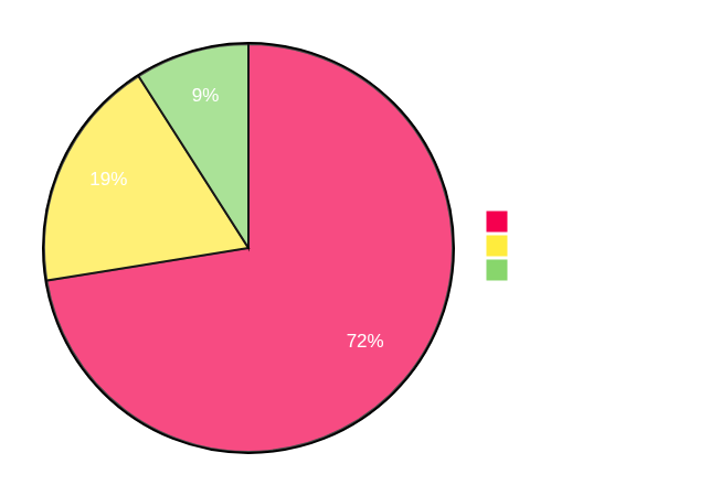
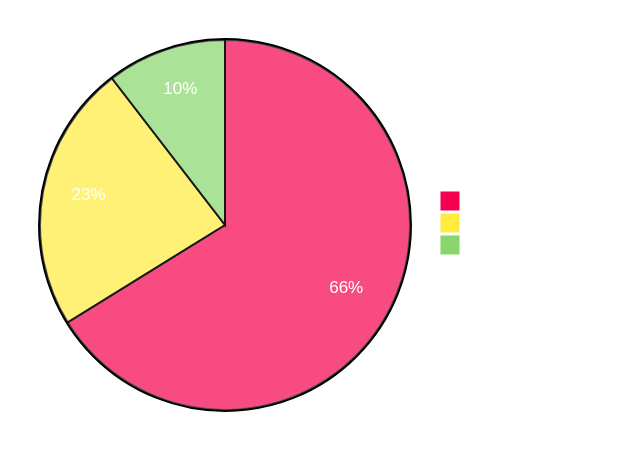
From game theoretic perspective, any air drop is a positive-sum game, i.e. there is no monetary loss even if the price of the tokens drops to zero. The utility is to derive the maximum profits. Consider a scenario where a new token launch has a vesting schedule of 20% at the time of launch and every quarter of the year, another 20%. So by the end of the year, all tokens would be vested.

Every user (U) is playing a game with the market (M). Each of them can either Sell (S) or Hold (H). Based on relative utility and the assumption that there will be more tokens available in the future, the following utility matrix resembles the outcome.

The effect of a user's action on the market is lower than a market's action on the user. Therefore, if both U and M sell at the time of air drop, they both derive the utility of (1,1). But if the U holds and M sells, there will be a much larger impact of that on user, hence their utility is (1, -3). If the U sells and M holds, there is a slightly higher utility for the user since they are selling at current holding price and hence we have (0,2). This can also be (0,1) and it would not make much difference. Important point to note here is that the action of holding gives a utility of 0 to both. People familiar with basics of Game Theory can quickly tell that there exists a pure-strategy Nash Equilibrium i.e. irrespective of what other player's actions are, your best strategy is to play the action with guaranteed maximum payoff. In our case, for both U and M, their best strategy is to Sell and get a payoff of (1,1).

This matrix is only valid when User knows that there are more tokens that will be available in the future. This is because all assets can theoretically gain value over time and it would be ideal to hold some portion with a certain probability of the protocol succeeding. Note that the last vesting schedule is identical to protocols with no vesting schedule as it then leaves it up to the user and their reasoning of the protocol's success. Which implies that all the vesting prior to the final one, simply gives more chance for users to dump their token.

From the protocol's perspective, this is disastrous. If the token price is somehow considered an indicator of the market's belief in protocol's success, then irrespective of how good the protocol is technically, it will get a bad rep. Furthermore, a non-vesting schedule air drop, entirely leaves it up to the market on how they perceive the protocol and let the market decide the optimal price point.

The reality​

If we look at most protocol's distribution of the tokens, majority are distributed to investors, core team and early adopters. For them, vesting or no-vesting should not make a difference and they would ideally Hold till the protocol gains some traction.

On the other hand, vesting still gives them disproportional power to start dumping at the most opportunistic moment, especially investors, whose major utility is realising profits over time. Don't get me wrong, I'm not trying to throw negative light on investors, I'm simply talking about their utility from a rational perspective.

Irrespective of how the newly vested tokens are distributed, new circulating supply decreases the FDV (Fully Diluted Valuations)and increases selling pressure. See a relevant report on Low Float, High FDV.

Any solution?​

Yes! A trivial sounding but not-so-trivial to implement on chains, is the idea of randomized vesting schedule. For each user, when the tokens will be vested is randomized. This creates a situation where a market cannot act in one way at one time because there is a fluctuating volume of tokens being vested every now and then.

For trading, randomized vesting schedules work to avoid nose dive of the token price. For governance, certain things need to be taken care of. Since all tokens are not vested at same time, a voting process should take into account all tokens, including the un-vested, to determine voting power (If the protocol uses one-token-one-vote mechanism).

So how can randomized vesting schedules be implemented? Through DVRFs! (Distributed Verifiable Random Function) The randomness from VRFs can be used to securely introduce random vesting schedule for each user.

ChainSafe R&D is currently working on implementing a better version of distributed verifiable random functions. More on that coming soon!

Recently, there has been a lot of excitement and interest around circle STARKs. This didn't pass me by either, and my interest was piqued. Not only by the loud "breakthrough" announcements and the prospects of unlocking verifiable computation on Bitcoin, but also by the subtle elegance of applied algebraic geometry to address limitations and simplify previous solutions.

At this point, we have several excellent introductory and explainer articles by zkSecurity, Vitalik, and LambdaClass. I have tried my best not to repeat their words and instead focus on the unexplored aspects and elements that I personally found very interesting. I wrote this as I was learning, so I cannot rule out inaccuracies. If you spot any mistakes, please comment away in this mirror on HackMD.

Introduction​

Circle STARKs enable the prover to work over the finite field modulo Mersenne 31 prime (M31), which has very efficient arithmetic. Namely, it is 1.3 times faster than BabyBear, the previous most efficient field used in SP1, Valida, and RISC Zero. For more insight on why working over M31 is so desirable, refer to this article.

However, simply plugging M31 into existing univariate STARKs won't work. The reason is that Mersenne primes are not FFT/FRI friendly. Let's unpack why.

The efficiency of the FFT "divide-and-conquer" algorithm relies on the ability to recursively divide the problem size by powers of 2. When working over a finite field, this requirement necessitates an evaluation domain to have the "structure" of a multiplicative group whose order's factorization contains a large power of two. We refer to this as high 2-adicity. The reason we want this is that at each step of the FFT, we reduce the size of the domain by a factor of two by squaring each number in it.

For example, consider the domain $[1, 85, 148, 111, 336, 252, 189, 226]$ in the finite field of integers modulo $337$. This domain forms a multiplicative group with $8 = 2^3$ elements. The elements of this group are powers of $\omega = 85$, which is a generator of the group. If you square every number in the domain, you reduce the size of the domain by a factor of two: $[1, 148, 111, 336]$. If you take the same domain but with, say, 6 elements, you don't get this property anymore.

Another relevant way of framing the 2-adicity requirement is to search for a group whose order is a product of small primes. We call such numbers smooth numbers. Since the multiplicative group of a field includes every element except $0$, the order of the group is exactly one less than the number of elements in the field. Fields $\mathbb{F}_p$ that satisfy this condition are referred to as $p-1$ smooth.

An exemplary prime is the BabyBear prime $p = 2^{31} - 2^{27} + 1$. The largest multiplicative group in the BabyBear field has $p-1 = 2^{27} \cdot 3 \cdot 5$ elements. You can clearly see that it is both smooth and highly 2-adic. It's perfect.

What about the Mersenne-31 prime $p = 2^{31} - 1$? Unfortunately, $2^{31} - 2$ can be divided by 2 only once. Thus, the conventional Cooley-Tukey FFT algorithm would be very inefficient for this field group. The authors solve this by devising a group from a unit circle.

Circle as a group​

A circle group is generated from a point $(x, y)$ such that $x^2 + y^2 = 1$ (i.e., it lies on a unit circle) by applying a different multiplicative law:

Instead of generating subgroup elements as simply powers of a generator $g$, we move from a point $(x_i, y_i)$ on the circle to the point:

It turns out that the number of points lying on the circle, defined over the Mersenne prime $2^{31}-1$, is quite large ($2^{31}$). One can generate all $2^{31}$ group elements by starting with $(x_0, y_0) = (1, 0)$ and applying the generator $(g_x, g_y) = (2, 1268011823)$ using the law above.

For the circle FFT/FRI, we need two more group operations: the group squaring map $\pi$ and the inversion map $J$.

Squaring is the quadratic map defined as

This transformation reduces the set size by half.

Inverse is given by the degree-one map

This operation maps each point $(x, y)$ to its reflection $(x, -y)$.

Map $J$ is an involution, i.e., $J(J(P)) = P$. Maps $J$ and $\pi$ commute, i.e., $\pi(J(P)) = J(\pi(P))$ for every $P \in C(\mathbb{F}_p)$.

FFT over the circle domain​

Same as in the classical STARK, the circle FFT is used to evaluate some polynomial on a special domain. In regular FFT, the domain consists of $n$-th roots of unity, i.e. $\{1, \omega, \omega^2, \ldots, \omega^{n-1}\}$. In circle FFT, the domain is a set of points on a circle curve, generated as follows.

First, we take a circle group generator $g$ and square it $\log n - 1$ times to create a subgroup $G_{n-1}$. Then, we create two twin cosets, which are formed by taking an element $Q$ that is not in $G_n$ and creating two disjoint sets: $Q \cdot G_{n-1}$ and $Q^{-1} \cdot G_{n-1}$. The union of these sets forms the circle FFT domain containing $2^n$ elements. A self-descriptive implementation can be found here in Plonky3.

An interactive plotter to demonstrate the distribution of domain points, which uses a simple TS implementation of the circle group over Mersenne-17 field. Even though it's modulo prime p, you can still see a regular circular patterns with symmetry about the line p/2. This phenomena is also exists in elliptic curves (genus 1), but is much more apparent on circle curves (genus 0) and complex roots of unity.

The FFT works by recursively splitting the larger problem into two smaller ones. In the context of polynomial evaluation, this means decomposing the polynomial into "even" and "odd" parts. In regular FFT, these sub-polynomials are simply formed from even and odd coefficients of the original polynomial. In circle FFT, this is a bit more involved, as we'll see, but the underlying mechanics is the same — the original polynomial $f$ is a linear combination $f(x) = f_{\operatorname{even}}(x) + x\cdot f_{\operatorname{odd}}(x)$. At each split, we also reduce the domain by a factor of two.

In the first step, we "halve" the domain by simply taking an $x$ projection of each point. This is justified by the use of the inverse map when performing a decomposition $f(x, y)=f_0(x)+y \cdot f_1(x)$ such that:

I have modified the notation to demonstrate how in practice we treat polynomials $f, f_0, f_1$ as vectors of their coefficients. Compare the original notation here with Vitalik's implementation here.

You can think of the inverse map $J(x, y) = (x, -y)$ as a way to identify vertically mirrored pairs of points so that they can be treated as a single entity. This allows us to proceed with only the $x$ coordinate.

In later steps, we continue to halve the domain using the univariate squaring map $\pi(x)=2 \cdot x^2-1$. This is analogous to squaring the $k$-th root of unity such that $\omega^{2k} = \omega_k$. The even-odd decomposition (in the original notation) $f_j(x) = f_{j+1}(\pi(x))+x \cdot f_{j+1}(\pi(x))$ — now looks like this:

Although speeding up the FFT is not the main point of the paper, as author points out here, it serves as an effective demonstration of the core principles of working over the circle group. When studying the paper, I made the mistake of skipping it and rushing to circle FRI only to hit a wall of confusion. So, I encourage you to take some time to appreciate this mechanic. If you want to play around with it, I made this Python notebook (trigger warning: shitty code).

Regular FRI​

Structure of the FRI algorithm is a lot like FFT. But instead of recursively dividing the polynomial into many smaller ones, in FRI, the prover iteratively reduces the degree of a polynomial until it gets to some small constant-size one. It does so via random linear combination, i.e., by combining "even" and "odd" sub-polynomials against a random weight.

In STARK, we use FRI for something called "low-degree testing"—by knowing the final degree and the number of reduction steps, the verifier can work backwards and check that the degree bound of the original polynomial is as claimed. More formally, FRI enables an untrusted prover to convince a verifier that a committed vector is close to a Reed-Solomon codeword of degree $d$ over the domain $D$.

Here, being "close" is defined by the relative Hamming distance $\delta$ such that the number of points where the committed vector and the codeword disagree is at most $\delta \cdot |D|$. The distance $\delta$ is such that $\delta \in (0,1-\sqrt{\rho})$ where $0 < \rho < 1$ is the rate of the Reed-Solomon code. In turn, the rate $\rho$ is defined by the blow-up factor $2^B, B \geq 1$ so that $\rho=2^{-B}$. Finally, the domain size is $|D| = 2^{n+B}$ where $2^n$ is the size of the original vector.

To make this definition more senseful, let's assign standard values: A commonly used blow-up factor is $2^B=4$, so the rate is $\rho = 0.25$. The worst possible distance is $\delta=0.5$, so for a vector with 1024 elements, the codeword over a $2^{B+n}=4096$ sized domain can disagree on at most half of the points. In practice, $\delta$ is much smaller to give better soundness guarantees.

Another interesting property is the decoding regime. In the unique decoding regime, the goal is to identify a single low-degree polynomial that is close to the committed vector. The unique decoding radius is typically defined as: $\theta \in [0, \frac{1-\rho}{2}]$.

STARKs are shown to be sound outside this regime as the goal is to demonstrate the existence of such polynomials, even if multiple polynomials fit the given points. We refer to this simplified requirement as the list decoding regime. The list decoding radius is typically defined as: $\theta \in [\frac{1-\rho}{2}, 1-\sqrt{\rho}]$. HAB23

Circle FRI​

The general mechanics behind low-degree testing over the circle domain remain unchanged from the regular FRI. As a reminder, see this blog post for an in-depth theoretical discussion or this one if you only care about the implementation.

Circle FRI operates on codewords in the circle code $\mathcal{C}$, which is a generalization of the Reed-Solomon code defined over elements of the circle group and special polynomials in Riemann-Roch space. Oversimplified, they are bivariate polynomials modulo the unit circle equation $(x^2 + y^2 = 1)$, so whenever a polynomial has $y^2$, it's replaced by $1 - x^2$.

For a given proximity parameter $\theta \in (0,1-\sqrt{\rho})$, the interactive oracle proof of a function $f: X \rightarrow \mathbb{F}^D$ (mapping the committed vector) being $\theta$-close to the circle codeword $\mathcal{C}$ consists of $r$ rounds of a commit phase and a subsequent query phase, which are as follows.

Commit phase​

1. $\mathbf{P}$ decomposes $f$ into $f=g+\lambda \cdot v_n$ and sends $\lambda$ to $\mathbf{V}$
2. $\mathbf{V}$ picks random weight $\lambda_j$ for layer $j$
3. For each $j=1, \ldots, r$, $\mathbf{P}$ decomposes $g_{j-1}$ into "even" and "odd" parts; sends a commitment $[g_j]$ to $\mathbf{V}$
4. In the last round, $\mathbf{P}$ sends $g_{r+1}$ in plain.

1. $\mathbf{P}$ decomposes $f$ into $f=g+\lambda \cdot v_n$ and sends $\lambda$ to $\mathbf{V}$​

We start with the extended domain coset $D_{n+B}$. First, we want to find the component of $f$ that is aligned with $v_n$. This can be done using vector projection: given two functions (or vectors) $f$ and $v_n$, the projection of $f$ onto $v_n$ is given by:

Note: angle brackets denote the inner product $\langle v_n, f\rangle_D=\sum_{x \in D} v_n(x) \cdot f(x)$.

Taking $\lambda$ as the magnitude of this projection will ensure that $\lambda \cdot v_n$ is the part of $f$ that lies along $v_n$

The vanishing polynomial $v_n$ has an alternating behavior over the domain $D$, e.g., if $D$ has size $N=2^n$, then $v_n$ alternates as $(1,-1,1,-1, \ldots)$. This significantly simplifies the inner product calculations as $v_n(x) \in \{1,-1\}$, each term $v_n(x)^2=1$ so

Knowing $\lambda$, we can now find $g$, which represents the component of $f$ that is orthogonal to $v_n$

This ensures that $g$ lies entirely in the FFT space $\mathcal{L}_N^{\prime}(F)$, orthogonal to $v_n$. This is because the inner product $\langle g, v_n\rangle_D=0$, making $g$ and $v_n$ orthogonal by construction.

2. $\mathbf{V}$ picks random weight $\lambda_j$ for layer $j$​

In practice, though, $\mathbf{P}$ can compute $\lambda_j$ as a random linear accumulator starting with $\lambda$ and using a single random weight $\alpha \in \mathbb{E}$ picked by $\mathbf{V}$

See this done in Stwo.

3. For each $j=1, \ldots, r$, $\mathbf{P}$ decomposes $g_{j-1}$ into "even" and "odd" parts​

The "even-odd" decomposition follows the same progression as in FFT. In the first round, we work with 2D points $(x, y)$ and use the full squaring $\pi(x, y)$ and inverse $J(x, y)$ maps. The inverse map transformation allows us to identify points $(x, y)$ and their reflection $(x, -y)$ so we can treat them as a single point $x$ on the $x$-axis in subsequent rounds. The squaring map $\pi$ transforms the domain $D_{j-1}$ into $D_j$ by effectively halving the space of points:

where $\pi(x)=2 \cdot x^2-1$ and $t_j$ is a twiddle factor. Then, fold into a random linear combination against $\lambda_j$:

Commitment $[g_j]$ is a simple Merkle root. Under the Fiat-Shamir transformation, $\mathbf{P}$ also sends openings, i.e., Merkle branches for FRI queries.

Query phase​

1. $\mathbf{V}$ samples $s \geq 1$ queries uniformly from the domain $D$​

For each query $Q$, $\mathbf{V}$ considers its "trace" as the sequence of points obtained by repeatedly applying the squaring map and the transformations defined by the protocol. The initial query point $Q_0=Q$ is transformed through several rounds, resulting in a series of points $Q_j$ in different domains $D_j$:

2. For each $j=1, \ldots, r$, $\mathbf{V}$ asks for the values of the function $g_j$ at a query point $Q_j$ and its reflection $T_j(Q_j)$​

Given the commitment $[g_j]$, as in oracle access, $\mathbf{V}$ can ask the oracle for the values (openings) at query points. In other words, verify Merkle proofs at the points:

where at $j=1$, $T_j=J$ and for $j>1$, $T_j(x)=-x$.

3. $\mathbf{V}$ checks that the returned values match the expected values according to the folding rules​

This involves checking that the even and odd decompositions are correct and that the random linear combinations used to form $g_j$ from $g_{j-1}$ are consistent.

DEEP quotients​

Quotienting is the fundamental polynomial identity check used in STARK and PLONKish systems. Leveraging the polynomial remainder theorem, it allows one to prove the value of a polynomial at a given point. Vitalik's overview of quotienting is well on point, so I will focus on the DEEP-FRI over the circle group.

DEEP (Domain Extension for Eliminating Pretenders) is a method for checking consistency between two polynomials by sampling a random point from a large domain. In layman's terms, it lets FRI be secure with fewer Merkle branches.

In STARK, we use the DEEP method on a relation between the constraint composition polynomial (one that combines all the constraints) and the trace column polynomials, all evaluated on a random point $z$. For more context, see this post and the ethSTARK paper.

The first part is DEEP algebraic linking: It allows us to reduce the STARK circuit satisfiability checks (for many columns and many constraints) to a low-degree test (FRI) on single-point quotients. By itself, DEEP-ALI is insecure because the prover can cheat and send inconsistent evaluations on $z$. We fix this with another instance of quotienting—DEEP quotienting.

We construct DEEP quotients with a single-point vanishing function $v_z$ in the denominator to show that a certain polynomial, say a trace column $t$, evaluates to the claim $y_j$ at $z$, i.e., $\frac{t - t(z)}{v_z}$.

In classical STARKs, $v_z$ is simply a line function $X - z$. In circle STARKs, in addition to not having line functions, we also run into the problem that single-point (or any odd degree) vanishing polynomials don't exist. To get around this, we move to the complex extension, i.e., decomposing into real and imaginary parts

Using with this quirk, we follow the standard procedure constructing a composite DEEP quotient polynomial as a random linear combination. We use different random weights for the real and imaginary parts

Computing $Q$ naïvely will suffer overhead due to the complex extension, essentially doubling the work due to real and imaginary decompositions. The authors solve this by exploiting the linearity in the above equation. The prover now computes

where $\bar{g}=\sum_{k=0}^{L-1} \gamma^k \cdot g_k$ and $\bar{v}_z=\sum_{k=0}^{L-1} \gamma^k \cdot g_k(z)$.

Interestingly, Stwo and Plonky3 actually use different quotienting approaches: Plonky3 implements the method described in the paper and here, but Stwo chooses instead to use a 2-point vanishing polynomial, as described in Vitalik's note.

Field work​

In circle STARK, work is done over the finite field $\mathbb{F}_p$ and its extension $\mathbb{E} = \mathbb{F}_{p^k}$ where $k$ is the extension degree. For $\mathbb{F}_p$, we choose M31, but any other $p+1$ smooth prime will suffice. The extension field $\mathbb{E}$ used in Stwo and Plonky3 is QM31, a degree-4 extension of M31, aka. the secure field.

In rare cases, it will be useful to work with the complex extension $\mathbb{F}(i)$, the field that results from $\mathbb{F}$ by extending it with the imaginary unit $i$. Note that $i$ may trivially be contained in some fields, e.g., if $-1 \equiv 4 \mod 5$ then $i$ in $\mathbb{F}_5$ is both $\sqrt{4} = 2$ and $3$ (since $2^3 \mod 5 \equiv 4$). For those fields where this isn't the case, such as $\mathbb{F}_3$, we can devise a quadratic extension, $\mathbb{F}_9 = \{ a + bi \mid a, b \in \mathbb{F}_3 \}$, which extends the original field in the same way complex numbers extend rationals.

• Trace values are over the base field and trace domain are points over the base field $\mathbb{C}(\mathbb{F})$.
• The evaluation domain consists of points over the base field $\mathbb{C}(\mathbb{F})$.
• All random challenges and weights for linear combinations are drawn from the secure field.
• When computing DEEP quotients, we move from the base field to secure fields, while briefly using complex extensions for vanishing denominators.
• Circle FRI works mainly on the secure field. However, query values are base field elements since we Merkle commit to values in the base field.

The results​

That's cool and all, but let's see how all this translates into actual performance differences. Below I have profiling charts comparing Plonky3 with regular STARK over BabyBear and circle STARK over M31.

The first thing to note is that the difference in prover time is indeed about 1.3x. You can see that circle STARK spends less time committing to the trace, as it does so over a more efficient base field. Consequently, since computing quotients and FRI involves extension field work, these are now account for a larger percentage of the total work.

Thanks to Shahar Papini for feedback and discussion.

References​

• [HLP24] Haböck et al. (2024) "Circle STARKs"
• [HAB23] Ulrich Haböck (2023) "A summary on the FRI low degree test"
• [ethSTARK] StarkWare Team (2023) "ethSTARK Documentation — Version 1.2"

Cryptographic work, such as commitments, is often the primary performance bottleneck in SNARKs. This cost is particularly pronounced when committed values are random and necessarily large, as is the case with PLONKish systems.

In recent years, a lot of innovation have been aimed at making commitments as cheap as possible. Circle STARKs and Binius, in particular, are hash-based and sound¹ over small fields, M31 and GF[2] respectively. This means lower prover overhead and better hardware compatibility.

However, it should be noted that FRI, the scheme behind these improvements, involves superlinear-time procedures like FFTs, which become a new bottleneck when applied directly to large computations without recursion.

In this note, I will explore GKR, an interactive proof (IP) scheme that addresses cryptographic overhead differently—by nearly avoiding commitments in the first place. My primary aim is to accurately summarize available materials and research. I am very open to changes and improvements, so if anything is unclear or incorrect, please leave comments here.

Background​

GKR08 is a relatively old scheme that is based on multivariate polynomials and the sum-check protocol. A technology that was largely ignored in favor of simpler designs featuring univariate polynomials and divisibility check. Lately, however, it has seen renewed interest as projects like Jolt, Expander, and Modulus have demonstrated not only its viability but also impressive performance results.

Notably, modern GKR-based systems demonstrate $O(n)$ prover complexity, which is linear in the size of the computation and with a constant factor overhead. For some applications, like matrix multiplication, the prover is less than 10x slower than a C++ program that simply evaluates the circuit, Tha13.

Furthermore, the aforementioned Binius is multivariate and it too involves sumcheck. Even StarkWare's Circle-Stark-based proof system called Stwo used GKR for LogUp lookups. I think it is safe to say that there is currently a broad consensus on the relevance of GKR.

Multilinear functions & MLEs​

Multilinear polynomial is a multivariate polynomial that is linear in each variable, meaning it has degree at most one in each variable. When multilinear polynomials defined over the boolean domain, they have a much lower degree compared to the univariate case for the same domain size, T23a.

For any multilinear polynomial $P\left(x_1, x_2, \ldots, x_v\right)$ over the boolean domain $\{0,1\}^v$ (the boolean hypercube), polynomial operations such as addition, multiplication, and evaluation can be performed using only the evaluations of $P$ on the boolean hypercube. This eliminates the need to explicitly reconstruct the polynomial from its evaluations, so there's no FFTs.

Multilinear extension (MLE) is used to translate functions into polynomials over the boolean domain $\{0,1\}^v$. Every function $f$ and vector $\vec{a}$ mapping from $\{0,1\}^v \rightarrow \mathbb{F}$ has exactly one extension polynomial that is multilinear.

The multilinear extension is a multivariate analog of the low-degree extensions (LDE) commonly present in STARKs. One thinks of $\operatorname{MLE}(f)$ as an "extension" of $a$, as $\operatorname{MLE}(a)$ "begins" with $a$ itself but includes a large number of additional entries. This distance-amplifying nature of MLE, combined with the Schwartz-Zippel lemma, forms the first basic building block of multivariate interactive proofs and GKR in particular.

Sumcheck​

The Sumcheck protocol allows a prover $\mathbf{P}$ to convince a verifier $\mathbf{V}$ that the sum of a multivariate polynomial over boolean inputs $[x_i \in \{0, 1\}]$ is computed correctly.

Sumcheck does not require $\mathbf{V}$ to know anything about the polynomial to which it is being applied. It is only until the final check in the protocol that, depending on the performance/succinctness tradeoff, $\mathbf{V}$ can choose to either request the polynomial and evaluate it directly or perform an oracle query, i.e., outsource the evaluation to $\mathbf{P}$ via a polynomial commitment scheme (PCS).

This is an interactive protocol: If $\ell$ is the number of variables in $g$, then $\ell$ rounds are required to complete the protocol. By applying the Fiat-Shamir transform, we can render the sumcheck non-interactive.

This post doesn't aim to explain the general workings of sumcheck. For that, I recommend T23a (section 4.1) or this blog post.

GKR​

In GKR, we work with layered circuits. A circuit is layered if it can be partitioned into layers such that every wire in the circuit is between adjacent layers, L23. The number of layers is the depth of the circuit, denoted as $d$. Note that many of today's variations of GKR allow for more arbitrary topologies just as well.

The arithmetic circuit $\mathcal{C}$ encodes logic with addition and multiplication gates to combine values on the incoming wires. Accordingly, functions $\operatorname{add}_i$ and $\operatorname{mul}_i$ are gate selectors that together constitute the wiring predicate of layer $i$.

We encode wire values on a boolean hypercube $\{0,1\}^n$, creating multi-linear extensions $\widetilde{W}_i(x)$ for each layer $i$. The output is in $\widetilde{W}_0(x)$, and inputs will be encoded in $\widetilde{W}_d(x)$.

Gate selectors depend only on the wiring pattern of the circuit, not on the values, so they can be evaluated by the verifier locally, XZZ19. Each gate $a$ at layer $i$ has two unique in-neighbors, namely $\operatorname{in}_1(a)$ and $\operatorname{in}_2(a)$.

and $\operatorname{mul}_i(a, b, c)=0$ for all $b, c \in\{0,1\}^{\ell_{i+1}}$ (the case where gate $a$ is a multiplication gate is similar), T23a. Selector MLEs are sparse, with at most $2^{2\ell}$ non-zero elements out of ${0,1}^{3\ell}$.

Note, the above definition does not reflect how selector MLEs are computed in practice, it is an effective method for illustrating the relationship between selectors and wire values.

The GKR prover starts with the output claim and iteratively applies the sumcheck protocol to reduce it from one layer to the next until it arrives at the input. The values on the layers are related thusly:

A few things to note here: First, notice how gate selectors are indexed—this aligns with the convention that selectors at layer $i$ determine how values from the next layer $i+1$ are combined. Notice also that the $i$-layer sumcheck is over boolean inputs of size $\ell_{i+1}$, i.e., the number of gates in the next layer.

Protocol​

1. $\mathbf{P}$ sends the output vector $\vec{\omega}$ and claims that $\tilde{\omega} = \widetilde{W}_0$.
2. $\mathbf{V}$ sends random $r_0 \in \mathbb{E}$ and computes $m_0 := \tilde{\omega}(r_0)$.
3. $\mathbf{P}$ and $\mathbf{V}$ apply sumcheck on the relation between $W_0$ and $W_1$ (using $f_{r_0}$ for the summand)
   $$\sum_{y, z \in\{0,1\}^{\ell_1}} f_{r_0}(y, z) \stackrel{?}{=} m_0$$
4. $\mathbf{P}$ and $\mathbf{V}$ reduce two claims $W_{i+1}(b)$ and $W_{i+1}(c)$ to a single random evaluation/combination $m_i$.
5. $\mathbf{P}$ and $\mathbf{V}$ apply sumcheck on the reduced relation $m_i$, alternating steps 4-5 for $d-1$ more times.
6. $\mathbf{V}$ checks that $\widetilde{W}_d$ is consistent with the inputs vector $\vec{x}$.

1. $\mathbf{P}$ sends the output vector $\vec{\omega}$ and claims that $\tilde{\omega} = \widetilde{W}_0$​

First, the $\mathbf{P}$ has to evaluate the circuit at the given input vector $\vec{x}$. This is why the prover is always at least linear to the size of the computation (circuit).

A common notation would be to write the output vector $\vec{\omega}$ as a function $D: \{0,1\}^{\ell_0} \rightarrow \mathbb{F}$ mapping output gate labels to output values, $2^{\ell_0}$ of them in total. The gate labels are the vertices of the boolean hypercube; for example, for $\ell_0=2$, the 4 output labels are $00$, $01$, $10$, $11$.

In practice, though, $\mathbf{P}$ and $\mathbf{V}$ work with polynomials, not functions, so they have to compute multilinear extension $\tilde{\omega}$ from the vector $\vec{\omega}$. Same goes for the inputs $\vec{x} \rightarrow \widetilde{W}_d$. However, since computation on MLEs can be performed over evaluations, in practice no additional computation, like interpolation/IFFT, is even required!

2. $\mathbf{V}$ sends random $r_0 \in \mathbb{E}$ and computes $m_0 := \tilde{\omega}(r_0)$​

$\mathbf{V}$ picks a random challenge $r_0 \in \mathbb{E}$. Crucially, the soundness error of the sumcheck protocol is inversely proportional to the size of the field from which challenges $r_i$ are drawn (due to the Schwartz-Zippel lemma), T23a. That's why in practice for challenge values, we use an extension field $\mathbb{E} := \mathbb{F}_{p^k}$ where $k$ is the extension degree.

For example, say we opt for M31 as a base field $\mathbb{F}_p$ whose order is $|\mathbb{F}_p| = p=2^{31}-1$ elements. Then, the probability of soundness error in sumcheck for an $\ell$-variate summand polynomial is $\frac{\ell}{2^{31}-1}$, which is too large, certainly for the non-interactive setting. Instead, we choose challenges from QM31—the extension field of M31 with $k=4$. Now, for any reasonable $\ell$, the soundness error can be considered negligible.

This soundness characteristic is a notable drawback of sumcheck-based systems, as it requires the GKR prover to work over extension fields after the second round, thus making field work the main contributor to the proving overhead. In Part 2, I'll cover the recent work from Bagad et al describing an algorithm that reduces the number of extension field operations by multiple orders of magnitude.

Also note that $\mathbf{V}$ cannot yet trust $\tilde{\omega}$ correctly to encode the outputs. The remainder of the protocol is devoted to confirming that the output claim is consistent with the rest of the circuit and its inputs.

3. $\mathbf{P}$ and $\mathbf{V}$ apply sumcheck on the relation between $W_0$ and $W_1$​

For the first layer, $\mathbf{P}$ and $\mathbf{V}$ run a sumcheck on Equation $(1)$ with $i=0$, between $W_0$ and $W_1$, with $x$ fixed to $r_0$.

In the first round of sumcheck, $\mathbf{P}$ uses $r_0$ to fix the variable $x$. In the remaining two rounds, $\mathbf{V}$ picks $b, c \in \mathbb{E}$ randomly to fix the variables $y$ and $z$, respectively. At the end of the sumcheck, from $\mathbf{V}$'s point of view, the relation on the sum (Equation $1$) is reduced to a simple check that the summand $f_{r_0}(b, c)$ evaluates to $m_0$.

To compute $f_{r_0}(b, c)$, $\mathbf{V}$ must compute $\operatorname{add}_{r_0}(b, c)$ and $\operatorname{mul}_{r_0}(b, c)$ locally. Remember that these depend only on the circuit's wiring pattern, not on the values. Since $f_{r_0}$ is recursive, $\mathbf{V}$ also asks $\mathbf{P}$ for the $\widetilde{W}_1(b)$ and $\widetilde{W}_1(c)$ values and computes $f_{r_0}(u, v)$ to complete the sumcheck protocol.

In this way, $\mathbf{P}$ and $\mathbf{V}$ reduce a claim about the output to two claims about values in layer 1. While $\mathbf{P}$ and $\mathbf{V}$ could recursively invoke two sumcheck protocols on $\widetilde{W}_1(b)$ and $\widetilde{W}_1(c)$ for the layers above, the number of claims and sumcheck protocols would grow exponentially in $d$. XZZ19

4. $\mathbf{P}$ and $\mathbf{V}$ reduce two claims $W_{i+1}(b)$ and $W_{i+1}(c)$ to a single random evaluation/combination $m_i$​

To avoid an exponential blow-up in complexity, $\mathbf{P}$ and $\mathbf{V}$ apply a "rand-eval" reduction subroutine.

Here I will describe a method from CFS17 based on random linear combination (RLC), as it is more commonly found in modern implementations. Later, for completeness, I will also include the method based on line restriction, as described in the original paper GKR08.

Given two claims $\widetilde{W}_1(b)$ and $\widetilde{W}_1(c)$, $\mathbf{V}$ picks random weights $\alpha_i, \beta_i \in \mathbb{E}$ and computes the RLC as

In the next step, $\mathbf{V}$ would use $m_i$ as the claim for the $i$-th layer sumcheck.

5. $\mathbf{P}$ and $\mathbf{V}$ apply sumcheck on the reduced relation $m_i$, alternating steps 4-5 for $d-1$ more times​

For the layers $i=1, \ldots, d-1$, $\mathbf{P}$ and $\mathbf{V}$ would execute the sumcheck protocol on Equation $(2)$ instead of Equation $(1)$

At the end of each layer's sumcheck protocol, $\mathbf{V}$ still receives two claims about $\widetilde{W}_{i+1}$, computes their random linear combination, and proceeds to the next layer above recursively until the input layer. XZZ19

6. $\mathbf{V}$ checks that $\widetilde{W}_d$ is consistent with the inputs vector $\vec{x}$​

At the input layer $d$, $\mathbf{V}$ receives two claims $\widetilde{W}_d(b_{i=d})$ and $\widetilde{W}_d(c_{i=d})$ from $\mathbf{P}$. Recall that $\widetilde{W}_d$ is claimed to be a multilinear extension of the input vector $\vec{x}$.

If $\mathbf{V}$ knows all the inputs in clear, they can compute $\widetilde{W}_d$ and evaluate it at $b_{i=d}$ and $c_{i=d}$ themselves.

Alternatively, if $\mathbf{V}$ doesn't know all inputs and is instead given an input commitment $[w_d]$ for succinctness or zero-knowledge reasons, then $\mathbf{V}$ queries the oracle for evaluations of $\widetilde{W}_d$ at $b_{i=d}$ and $c_{i=d}$.

Ultimately, $\mathbf{V}$ outputs $\mathbf{accept}$ if the evaluated values are the same as the two claims; otherwise, they output $\mathbf{reject}$. XZZ19

Analysis​

Let $\mathcal{C}: \mathbb{F} \rightarrow \mathbb{E}$ be a layered circuit of depth $d$ with $n := |\vec{x}|$ input variables, having $S_i$ gates in layer $i$. Naturally, $|\mathcal{C}| := \sum^d_{i=0} S_i$ is the total number of gates in the circuit, i.e., the circuit size.

• Rounds: $O(d\cdot \log |\mathcal{C}|)$.
• $\mathbf{P}$ time: $O(|\mathcal{C}|\cdot\log |\mathcal{C}|)$
• $\mathbf{V}$ work: $O(n+d\cdot\log |\mathcal{C}|+t+S_0) \approx O(n+d\cdot\log |\mathcal{C}|)$ for 1 output.
• Communication: $O(S_0+d\cdot\log |\mathcal{C}|)$ field elements.
• Soundness error: $O(\frac{d\cdot\log |\mathcal{C}|}{|\mathbb{E}|})$

The GKR protocol consists of one execution of the sumcheck protocol per layer. Therefore, the total communication cost (proof size) is $O(d \log |\mathcal{C}|)$ field elements. The accumulated soundness error is $O\left(\frac{d \cdot \log |\mathcal{C}|}{|\mathbb{E}|}\right)$ due to the Schwartz-Zippel lemma. T23a

The prover must first evaluate the circuit, which takes time $|\mathcal{C}|$. It must also compute $\operatorname{add}_i$ and $\operatorname{mul}_i$ at each layer, which, if done trivially, induces logarithmic overhead $\log |\mathcal{C}|$. The resulting time for the prover is $O(|\mathcal{C}| \cdot \log |\mathcal{C}|)$. XZZ19

The verifier's work is $O(n + d \log |\mathcal{C}| + t + S_0)$, where $S_0$ is the number of outputs of the circuit, $t$ denotes the optimal time to evaluate all $\operatorname{add}_i$ and $\operatorname{mul}_i$, and the $n$ term is due to the time needed to evaluate $\widetilde{W}_d$. XZZ19

Part 2 will cover modifications and techniques that result in $O(|\mathcal{C}|)$ prover.

Zero Knowledge​

To make the sumcheck protocol zero-knowledge, the polynomial in the sumcheck protocol is masked by a random polynomial.

To prove the sumcheck for the summand polynomial $f$ from Equation $(1)$ and a claim $W$ in zero-knowledge, $\mathbf{P}$ generates a random polynomial $\gamma$ with the same variables and individual degrees as $f$, commits to $\gamma$, and sends $\mathbf{V}$ a claim $\Gamma = \sum_{x_1, \ldots, x_{\ell} \in \{0,1\}^{\ell}} \gamma(x_1, \ldots, x_{\ell})$ $\mathbf{V}$ picks a random number $\rho$, and together with $\mathbf{P}$ executes the sumcheck protocol on

In the last round of this sumcheck, $\mathbf{P}$ opens the commitment to $\gamma$ at $\gamma(r_1, \ldots, r_{\ell})$, and the verifier computes $f(r_1, \ldots, r_{\ell})$ by subtracting $\rho \cdot \gamma(r_1, \ldots, r_{\ell})$ from the last message, and compares it with $\mathbf{P}$'s original claim.

Chiesa et al. showed that as long as the commitment and opening of $\gamma$ are zero-knowledge, the protocol is zero-knowledge.

Original method to reduce two claims to one​

Let $\widetilde{W}$ be a multilinear polynomial over $\mathbb{F}$ with $\log n$ variables. The following is the description of a simple one-round subroutine from GKR08 with communication cost $O(\log n)$ that reduces the evaluation of $\widetilde{W}(b)$ and $\widetilde{W}(c)$ to the evaluation of $\widetilde{W}(r)$ for a single point $r \in \mathbb{E}$.

$\mathbf{P}$ interpolates a unique line $\ell$ passing through $b$ and $c$, such that $\ell(0)=b$ and $\ell(1)=c$. The line can be formally defined as $\ell(t) = b + t \cdot (c - b)$ using the point-slope form. The points $b$ and $c$ are tuples with $v$ elements for a $v$-variate polynomial $\widetilde{W}$.

By substituting $b$ and $c - b$ into $\ell(t)$, we get the tuple $\ell(t) = (\ell_0(t), \cdots, \ell_{v}(t))$ defined by $v$ linear polynomials over $t$. $\mathbf{P}$ sends a univariate polynomial $q$ of degree at most $k_{i+1}$ that is claimed to be $\widetilde{W}_{i+1} \circ \ell$, the restriction of $\widetilde{W}_{i+1}$ to the unique line $\ell$.