Recently, there has been a lot of excitement and interest around circle STARKs. This didn't pass me by either, and my interest was piqued. Not only by the loud "breakthrough" announcements and the prospects of unlocking verifiable computation on Bitcoin, but also by the subtle elegance of applied algebraic geometry to address limitations and simplify previous solutions.

At this point, we have several excellent introductory and explainer articles by zkSecurity, Vitalik, and LambdaClass. I have tried my best not to repeat their words and instead focus on the unexplored aspects and elements that I personally found very interesting. I wrote this as I was learning, so I cannot rule out inaccuracies. If you spot any mistakes, please comment away in this mirror on HackMD.

Introduction​

Circle STARKs enable the prover to work over the finite field modulo Mersenne 31 prime (M31), which has very efficient arithmetic. Namely, it is 1.3 times faster than BabyBear, the previous most efficient field used in SP1, Valida, and RISC Zero. For more insight on why working over M31 is so desirable, refer to this article.

However, simply plugging M31 into existing univariate STARKs won't work. The reason is that Mersenne primes are not FFT/FRI friendly. Let's unpack why.

The efficiency of the FFT "divide-and-conquer" algorithm relies on the ability to recursively divide the problem size by powers of 2. When working over a finite field, this requirement necessitates an evaluation domain to have the "structure" of a multiplicative group whose order's factorization contains a large power of two. We refer to this as high 2-adicity. The reason we want this is that at each step of the FFT, we reduce the size of the domain by a factor of two by squaring each number in it.

For example, consider the domain $[1, 85, 148, 111, 336, 252, 189, 226]$ in the finite field of integers modulo $337$. This domain forms a multiplicative group with $8 = 2^3$ elements. The elements of this group are powers of $\omega = 85$, which is a generator of the group. If you square every number in the domain, you reduce the size of the domain by a factor of two: $[1, 148, 111, 336]$. If you take the same domain but with, say, 6 elements, you don't get this property anymore.

Another relevant way of framing the 2-adicity requirement is to search for a group whose order is a product of small primes. We call such numbers smooth numbers. Since the multiplicative group of a field includes every element except $0$, the order of the group is exactly one less than the number of elements in the field. Fields $\mathbb{F}_p$ that satisfy this condition are referred to as $p-1$ smooth.

An exemplary prime is the BabyBear prime $p = 2^{31} - 2^{27} + 1$. The largest multiplicative group in the BabyBear field has $p-1 = 2^{27} \cdot 3 \cdot 5$ elements. You can clearly see that it is both smooth and highly 2-adic. It's perfect.

What about the Mersenne-31 prime $p = 2^{31} - 1$? Unfortunately, $2^{31} - 2$ can be divided by 2 only once. Thus, the conventional Cooley-Tukey FFT algorithm would be very inefficient for this field group. The authors solve this by devising a group from a unit circle.

Circle as a group​

A circle group is generated from a point $(x, y)$ such that $x^2 + y^2 = 1$ (i.e., it lies on a unit circle) by applying a different multiplicative law:

Instead of generating subgroup elements as simply powers of a generator $g$, we move from a point $(x_i, y_i)$ on the circle to the point:

It turns out that the number of points lying on the circle, defined over the Mersenne prime $2^{31}-1$, is quite large ($2^{31}$). One can generate all $2^{31}$ group elements by starting with $(x_0, y_0) = (1, 0)$ and applying the generator $(g_x, g_y) = (2, 1268011823)$ using the law above.

For the circle FFT/FRI, we need two more group operations: the group squaring map $\pi$ and the inversion map $J$.

Squaring is the quadratic map defined as

This transformation reduces the set size by half.

Inverse is given by the degree-one map

This operation maps each point $(x, y)$ to its reflection $(x, -y)$.

Map $J$ is an involution, i.e., $J(J(P)) = P$. Maps $J$ and $\pi$ commute, i.e., $\pi(J(P)) = J(\pi(P))$ for every $P \in C(\mathbb{F}_p)$.

FFT over the circle domain​

Same as in the classical STARK, the circle FFT is used to evaluate some polynomial on a special domain. In regular FFT, the domain consists of $n$-th roots of unity, i.e. $\{1, \omega, \omega^2, \ldots, \omega^{n-1}\}$. In circle FFT, the domain is a set of points on a circle curve, generated as follows.

First, we take a circle group generator $g$ and square it $\log n - 1$ times to create a subgroup $G_{n-1}$. Then, we create two twin cosets, which are formed by taking an element $Q$ that is not in $G_n$ and creating two disjoint sets: $Q \cdot G_{n-1}$ and $Q^{-1} \cdot G_{n-1}$. The union of these sets forms the circle FFT domain containing $2^n$ elements. A self-descriptive implementation can be found here in Plonky3.

An interactive plotter to demonstrate the distribution of domain points, which uses a simple TS implementation of the circle group over Mersenne-17 field. Even though it's modulo prime p, you can still see a regular circular patterns with symmetry about the line p/2. This phenomena is also exists in elliptic curves (genus 1), but is much more apparent on circle curves (genus 0) and complex roots of unity.

The FFT works by recursively splitting the larger problem into two smaller ones. In the context of polynomial evaluation, this means decomposing the polynomial into "even" and "odd" parts. In regular FFT, these sub-polynomials are simply formed from even and odd coefficients of the original polynomial. In circle FFT, this is a bit more involved, as we'll see, but the underlying mechanics is the same — the original polynomial $f$ is a linear combination $f(x) = f_{\operatorname{even}}(x) + x\cdot f_{\operatorname{odd}}(x)$. At each split, we also reduce the domain by a factor of two.

In the first step, we "halve" the domain by simply taking an $x$ projection of each point. This is justified by the use of the inverse map when performing a decomposition $f(x, y)=f_0(x)+y \cdot f_1(x)$ such that:

I have modified the notation to demonstrate how in practice we treat polynomials $f, f_0, f_1$ as vectors of their coefficients. Compare the original notation here with Vitalik's implementation here.

You can think of the inverse map $J(x, y) = (x, -y)$ as a way to identify vertically mirrored pairs of points so that they can be treated as a single entity. This allows us to proceed with only the $x$ coordinate.

In later steps, we continue to halve the domain using the univariate squaring map $\pi(x)=2 \cdot x^2-1$. This is analogous to squaring the $k$-th root of unity such that $\omega^{2k} = \omega_k$. The even-odd decomposition (in the original notation) $f_j(x) = f_{j+1}(\pi(x))+x \cdot f_{j+1}(\pi(x))$ — now looks like this:

Although speeding up the FFT is not the main point of the paper, as author points out here, it serves as an effective demonstration of the core principles of working over the circle group. When studying the paper, I made the mistake of skipping it and rushing to circle FRI only to hit a wall of confusion. So, I encourage you to take some time to appreciate this mechanic. If you want to play around with it, I made this Python notebook (trigger warning: shitty code).

Regular FRI​

Structure of the FRI algorithm is a lot like FFT. But instead of recursively dividing the polynomial into many smaller ones, in FRI, the prover iteratively reduces the degree of a polynomial until it gets to some small constant-size one. It does so via random linear combination, i.e., by combining "even" and "odd" sub-polynomials against a random weight.

In STARK, we use FRI for something called "low-degree testing"—by knowing the final degree and the number of reduction steps, the verifier can work backwards and check that the degree bound of the original polynomial is as claimed. More formally, FRI enables an untrusted prover to convince a verifier that a committed vector is close to a Reed-Solomon codeword of degree $d$ over the domain $D$.

Here, being "close" is defined by the relative Hamming distance $\delta$ such that the number of points where the committed vector and the codeword disagree is at most $\delta \cdot |D|$. The distance $\delta$ is such that $\delta \in (0,1-\sqrt{\rho})$ where $0 < \rho < 1$ is the rate of the Reed-Solomon code. In turn, the rate $\rho$ is defined by the blow-up factor $2^B, B \geq 1$ so that $\rho=2^{-B}$. Finally, the domain size is $|D| = 2^{n+B}$ where $2^n$ is the size of the original vector.

To make this definition more senseful, let's assign standard values: A commonly used blow-up factor is $2^B=4$, so the rate is $\rho = 0.25$. The worst possible distance is $\delta=0.5$, so for a vector with 1024 elements, the codeword over a $2^{B+n}=4096$ sized domain can disagree on at most half of the points. In practice, $\delta$ is much smaller to give better soundness guarantees.

Another interesting property is the decoding regime. In the unique decoding regime, the goal is to identify a single low-degree polynomial that is close to the committed vector. The unique decoding radius is typically defined as: $\theta \in [0, \frac{1-\rho}{2}]$.

STARKs are shown to be sound outside this regime as the goal is to demonstrate the existence of such polynomials, even if multiple polynomials fit the given points. We refer to this simplified requirement as the list decoding regime. The list decoding radius is typically defined as: $\theta \in [\frac{1-\rho}{2}, 1-\sqrt{\rho}]$. HAB23

Circle FRI​

The general mechanics behind low-degree testing over the circle domain remain unchanged from the regular FRI. As a reminder, see this blog post for an in-depth theoretical discussion or this one if you only care about the implementation.

Circle FRI operates on codewords in the circle code $\mathcal{C}$, which is a generalization of the Reed-Solomon code defined over elements of the circle group and special polynomials in Riemann-Roch space. Oversimplified, they are bivariate polynomials modulo the unit circle equation $(x^2 + y^2 = 1)$, so whenever a polynomial has $y^2$, it's replaced by $1 - x^2$.

For a given proximity parameter $\theta \in (0,1-\sqrt{\rho})$, the interactive oracle proof of a function $f: X \rightarrow \mathbb{F}^D$ (mapping the committed vector) being $\theta$-close to the circle codeword $\mathcal{C}$ consists of $r$ rounds of a commit phase and a subsequent query phase, which are as follows.

Commit phase​

1. $\mathbf{P}$ decomposes $f$ into $f=g+\lambda \cdot v_n$ and sends $\lambda$ to $\mathbf{V}$
2. $\mathbf{V}$ picks random weight $\lambda_j$ for layer $j$
3. For each $j=1, \ldots, r$, $\mathbf{P}$ decomposes $g_{j-1}$ into "even" and "odd" parts; sends a commitment $[g_j]$ to $\mathbf{V}$
4. In the last round, $\mathbf{P}$ sends $g_{r+1}$ in plain.

1. $\mathbf{P}$ decomposes $f$ into $f=g+\lambda \cdot v_n$ and sends $\lambda$ to $\mathbf{V}$​

We start with the extended domain coset $D_{n+B}$. First, we want to find the component of $f$ that is aligned with $v_n$. This can be done using vector projection: given two functions (or vectors) $f$ and $v_n$, the projection of $f$ onto $v_n$ is given by:

Note: angle brackets denote the inner product $\langle v_n, f\rangle_D=\sum_{x \in D} v_n(x) \cdot f(x)$.

Taking $\lambda$ as the magnitude of this projection will ensure that $\lambda \cdot v_n$ is the part of $f$ that lies along $v_n$

The vanishing polynomial $v_n$ has an alternating behavior over the domain $D$, e.g., if $D$ has size $N=2^n$, then $v_n$ alternates as $(1,-1,1,-1, \ldots)$. This significantly simplifies the inner product calculations as $v_n(x) \in \{1,-1\}$, each term $v_n(x)^2=1$ so

Knowing $\lambda$, we can now find $g$, which represents the component of $f$ that is orthogonal to $v_n$

This ensures that $g$ lies entirely in the FFT space $\mathcal{L}_N^{\prime}(F)$, orthogonal to $v_n$. This is because the inner product $\langle g, v_n\rangle_D=0$, making $g$ and $v_n$ orthogonal by construction.

2. $\mathbf{V}$ picks random weight $\lambda_j$ for layer $j$​

In practice, though, $\mathbf{P}$ can compute $\lambda_j$ as a random linear accumulator starting with $\lambda$ and using a single random weight $\alpha \in \mathbb{E}$ picked by $\mathbf{V}$

See this done in Stwo.

3. For each $j=1, \ldots, r$, $\mathbf{P}$ decomposes $g_{j-1}$ into "even" and "odd" parts​

The "even-odd" decomposition follows the same progression as in FFT. In the first round, we work with 2D points $(x, y)$ and use the full squaring $\pi(x, y)$ and inverse $J(x, y)$ maps. The inverse map transformation allows us to identify points $(x, y)$ and their reflection $(x, -y)$ so we can treat them as a single point $x$ on the $x$-axis in subsequent rounds. The squaring map $\pi$ transforms the domain $D_{j-1}$ into $D_j$ by effectively halving the space of points:

where $\pi(x)=2 \cdot x^2-1$ and $t_j$ is a twiddle factor. Then, fold into a random linear combination against $\lambda_j$:

Commitment $[g_j]$ is a simple Merkle root. Under the Fiat-Shamir transformation, $\mathbf{P}$ also sends openings, i.e., Merkle branches for FRI queries.

Query phase​

1. $\mathbf{V}$ samples $s \geq 1$ queries uniformly from the domain $D$​

For each query $Q$, $\mathbf{V}$ considers its "trace" as the sequence of points obtained by repeatedly applying the squaring map and the transformations defined by the protocol. The initial query point $Q_0=Q$ is transformed through several rounds, resulting in a series of points $Q_j$ in different domains $D_j$:

2. For each $j=1, \ldots, r$, $\mathbf{V}$ asks for the values of the function $g_j$ at a query point $Q_j$ and its reflection $T_j(Q_j)$​

Given the commitment $[g_j]$, as in oracle access, $\mathbf{V}$ can ask the oracle for the values (openings) at query points. In other words, verify Merkle proofs at the points:

where at $j=1$, $T_j=J$ and for $j>1$, $T_j(x)=-x$.

3. $\mathbf{V}$ checks that the returned values match the expected values according to the folding rules​

This involves checking that the even and odd decompositions are correct and that the random linear combinations used to form $g_j$ from $g_{j-1}$ are consistent.

DEEP quotients​

Quotienting is the fundamental polynomial identity check used in STARK and PLONKish systems. Leveraging the polynomial remainder theorem, it allows one to prove the value of a polynomial at a given point. Vitalik's overview of quotienting is well on point, so I will focus on the DEEP-FRI over the circle group.

DEEP (Domain Extension for Eliminating Pretenders) is a method for checking consistency between two polynomials by sampling a random point from a large domain. In layman's terms, it lets FRI be secure with fewer Merkle branches.

In STARK, we use the DEEP method on a relation between the constraint composition polynomial (one that combines all the constraints) and the trace column polynomials, all evaluated on a random point $z$. For more context, see this post and the ethSTARK paper.

The first part is DEEP algebraic linking: It allows us to reduce the STARK circuit satisfiability checks (for many columns and many constraints) to a low-degree test (FRI) on single-point quotients. By itself, DEEP-ALI is insecure because the prover can cheat and send inconsistent evaluations on $z$. We fix this with another instance of quotienting—DEEP quotienting.

We construct DEEP quotients with a single-point vanishing function $v_z$ in the denominator to show that a certain polynomial, say a trace column $t$, evaluates to the claim $y_j$ at $z$, i.e., $\frac{t - t(z)}{v_z}$.

In classical STARKs, $v_z$ is simply a line function $X - z$. In circle STARKs, in addition to not having line functions, we also run into the problem that single-point (or any odd degree) vanishing polynomials don't exist. To get around this, we move to the complex extension, i.e., decomposing into real and imaginary parts

Using with this quirk, we follow the standard procedure constructing a composite DEEP quotient polynomial as a random linear combination. We use different random weights for the real and imaginary parts

Computing $Q$ naïvely will suffer overhead due to the complex extension, essentially doubling the work due to real and imaginary decompositions. The authors solve this by exploiting the linearity in the above equation. The prover now computes

where $\bar{g}=\sum_{k=0}^{L-1} \gamma^k \cdot g_k$ and $\bar{v}_z=\sum_{k=0}^{L-1} \gamma^k \cdot g_k(z)$.

Interestingly, Stwo and Plonky3 actually use different quotienting approaches: Plonky3 implements the method described in the paper and here, but Stwo chooses instead to use a 2-point vanishing polynomial, as described in Vitalik's note.

Field work​

In circle STARK, work is done over the finite field $\mathbb{F}_p$ and its extension $\mathbb{E} = \mathbb{F}_{p^k}$ where $k$ is the extension degree. For $\mathbb{F}_p$, we choose M31, but any other $p+1$ smooth prime will suffice. The extension field $\mathbb{E}$ used in Stwo and Plonky3 is QM31, a degree-4 extension of M31, aka. the secure field.

In rare cases, it will be useful to work with the complex extension $\mathbb{F}(i)$, the field that results from $\mathbb{F}$ by extending it with the imaginary unit $i$. Note that $i$ may trivially be contained in some fields, e.g., if $-1 \equiv 4 \mod 5$ then $i$ in $\mathbb{F}_5$ is both $\sqrt{4} = 2$ and $3$ (since $2^3 \mod 5 \equiv 4$). For those fields where this isn't the case, such as $\mathbb{F}_3$, we can devise a quadratic extension, $\mathbb{F}_9 = \{ a + bi \mid a, b \in \mathbb{F}_3 \}$, which extends the original field in the same way complex numbers extend rationals.

• Trace values are over the base field and trace domain are points over the base field $\mathbb{C}(\mathbb{F})$.
• The evaluation domain consists of points over the base field $\mathbb{C}(\mathbb{F})$.
• All random challenges and weights for linear combinations are drawn from the secure field.
• When computing DEEP quotients, we move from the base field to secure fields, while briefly using complex extensions for vanishing denominators.
• Circle FRI works mainly on the secure field. However, query values are base field elements since we Merkle commit to values in the base field.

The results​

That's cool and all, but let's see how all this translates into actual performance differences. Below I have profiling charts comparing Plonky3 with regular STARK over BabyBear and circle STARK over M31.

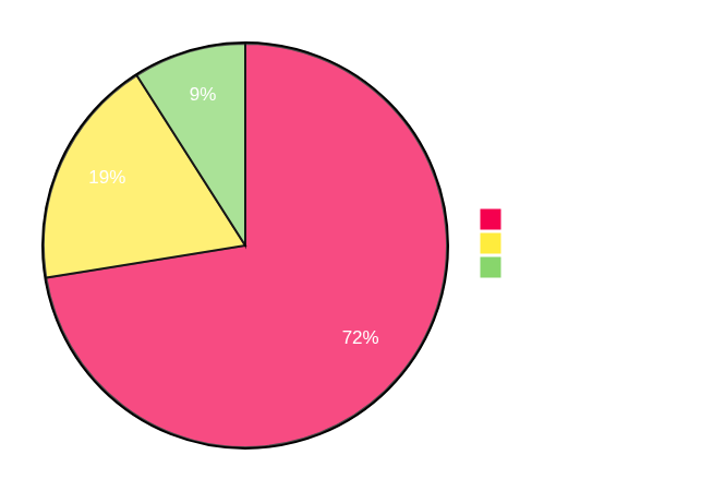
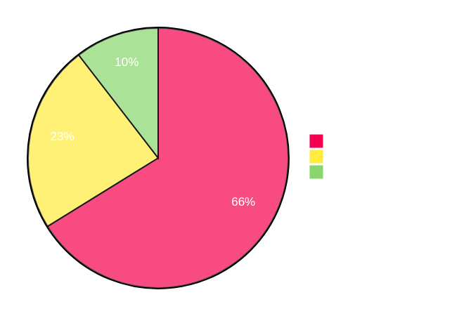
The first thing to note is that the difference in prover time is indeed about 1.3x. You can see that circle STARK spends less time committing to the trace, as it does so over a more efficient base field. Consequently, since computing quotients and FRI involves extension field work, these are now account for a larger percentage of the total work.

Thanks to Shahar Papini for feedback and discussion.

References​

• [HLP24] Haböck et al. (2024) "Circle STARKs"
• [HAB23] Ulrich Haböck (2023) "A summary on the FRI low degree test"
• [ethSTARK] StarkWare Team (2023) "ethSTARK Documentation — Version 1.2"

Cryptographic work, such as commitments, is often the primary performance bottleneck in SNARKs. This cost is particularly pronounced when committed values are random and necessarily large, as is the case with PLONKish systems.

In recent years, a lot of innovation have been aimed at making commitments as cheap as possible. Circle STARKs and Binius, in particular, are hash-based and sound¹ over small fields, M31 and GF[2] respectively. This means lower prover overhead and better hardware compatibility.

However, it should be noted that FRI, the scheme behind these improvements, involves superlinear-time procedures like FFTs, which become a new bottleneck when applied directly to large computations without recursion.

In this note, I will explore GKR, an interactive proof (IP) scheme that addresses cryptographic overhead differently—by nearly avoiding commitments in the first place. My primary aim is to accurately summarize available materials and research. I am very open to changes and improvements, so if anything is unclear or incorrect, please leave comments here.

Background​

GKR08 is a relatively old scheme that is based on multivariate polynomials and the sum-check protocol. A technology that was largely ignored in favor of simpler designs featuring univariate polynomials and divisibility check. Lately, however, it has seen renewed interest as projects like Jolt, Expander, and Modulus have demonstrated not only its viability but also impressive performance results.

Notably, modern GKR-based systems demonstrate $O(n)$ prover complexity, which is linear in the size of the computation and with a constant factor overhead. For some applications, like matrix multiplication, the prover is less than 10x slower than a C++ program that simply evaluates the circuit, Tha13.

Furthermore, the aforementioned Binius is multivariate and it too involves sumcheck. Even StarkWare's Circle-Stark-based proof system called Stwo used GKR for LogUp lookups. I think it is safe to say that there is currently a broad consensus on the relevance of GKR.

Multilinear functions & MLEs​

Multilinear polynomial is a multivariate polynomial that is linear in each variable, meaning it has degree at most one in each variable. When multilinear polynomials defined over the boolean domain, they have a much lower degree compared to the univariate case for the same domain size, T23a.

For any multilinear polynomial $P\left(x_1, x_2, \ldots, x_v\right)$ over the boolean domain $\{0,1\}^v$ (the boolean hypercube), polynomial operations such as addition, multiplication, and evaluation can be performed using only the evaluations of $P$ on the boolean hypercube. This eliminates the need to explicitly reconstruct the polynomial from its evaluations, so there's no FFTs.

Multilinear extension (MLE) is used to translate functions into polynomials over the boolean domain $\{0,1\}^v$. Every function $f$ and vector $\vec{a}$ mapping from $\{0,1\}^v \rightarrow \mathbb{F}$ has exactly one extension polynomial that is multilinear.

The multilinear extension is a multivariate analog of the low-degree extensions (LDE) commonly present in STARKs. One thinks of $\operatorname{MLE}(f)$ as an "extension" of $a$, as $\operatorname{MLE}(a)$ "begins" with $a$ itself but includes a large number of additional entries. This distance-amplifying nature of MLE, combined with the Schwartz-Zippel lemma, forms the first basic building block of multivariate interactive proofs and GKR in particular.

Sumcheck​

The Sumcheck protocol allows a prover $\mathbf{P}$ to convince a verifier $\mathbf{V}$ that the sum of a multivariate polynomial over boolean inputs $[x_i \in \{0, 1\}]$ is computed correctly.

Sumcheck does not require $\mathbf{V}$ to know anything about the polynomial to which it is being applied. It is only until the final check in the protocol that, depending on the performance/succinctness tradeoff, $\mathbf{V}$ can choose to either request the polynomial and evaluate it directly or perform an oracle query, i.e., outsource the evaluation to $\mathbf{P}$ via a polynomial commitment scheme (PCS).

This is an interactive protocol: If $\ell$ is the number of variables in $g$, then $\ell$ rounds are required to complete the protocol. By applying the Fiat-Shamir transform, we can render the sumcheck non-interactive.

This post doesn't aim to explain the general workings of sumcheck. For that, I recommend T23a (section 4.1) or this blog post.

GKR​

In GKR, we work with layered circuits. A circuit is layered if it can be partitioned into layers such that every wire in the circuit is between adjacent layers, L23. The number of layers is the depth of the circuit, denoted as $d$. Note that many of today's variations of GKR allow for more arbitrary topologies just as well.

The arithmetic circuit $\mathcal{C}$ encodes logic with addition and multiplication gates to combine values on the incoming wires. Accordingly, functions $\operatorname{add}_i$ and $\operatorname{mul}_i$ are gate selectors that together constitute the wiring predicate of layer $i$.

We encode wire values on a boolean hypercube $\{0,1\}^n$, creating multi-linear extensions $\widetilde{W}_i(x)$ for each layer $i$. The output is in $\widetilde{W}_0(x)$, and inputs will be encoded in $\widetilde{W}_d(x)$.

Gate selectors depend only on the wiring pattern of the circuit, not on the values, so they can be evaluated by the verifier locally, XZZ19. Each gate $a$ at layer $i$ has two unique in-neighbors, namely $\operatorname{in}_1(a)$ and $\operatorname{in}_2(a)$.

and $\operatorname{mul}_i(a, b, c)=0$ for all $b, c \in\{0,1\}^{\ell_{i+1}}$ (the case where gate $a$ is a multiplication gate is similar), T23a. Selector MLEs are sparse, with at most $2^{2\ell}$ non-zero elements out of ${0,1}^{3\ell}$.

Note, the above definition does not reflect how selector MLEs are computed in practice, it is an effective method for illustrating the relationship between selectors and wire values.

The GKR prover starts with the output claim and iteratively applies the sumcheck protocol to reduce it from one layer to the next until it arrives at the input. The values on the layers are related thusly:

A few things to note here: First, notice how gate selectors are indexed—this aligns with the convention that selectors at layer $i$ determine how values from the next layer $i+1$ are combined. Notice also that the $i$-layer sumcheck is over boolean inputs of size $\ell_{i+1}$, i.e., the number of gates in the next layer.

Protocol​

1. $\mathbf{P}$ sends the output vector $\vec{\omega}$ and claims that $\tilde{\omega} = \widetilde{W}_0$.
2. $\mathbf{V}$ sends random $r_0 \in \mathbb{E}$ and computes $m_0 := \tilde{\omega}(r_0)$.
3. $\mathbf{P}$ and $\mathbf{V}$ apply sumcheck on the relation between $W_0$ and $W_1$ (using $f_{r_0}$ for the summand)
   $$\sum_{y, z \in\{0,1\}^{\ell_1}} f_{r_0}(y, z) \stackrel{?}{=} m_0$$
4. $\mathbf{P}$ and $\mathbf{V}$ reduce two claims $W_{i+1}(b)$ and $W_{i+1}(c)$ to a single random evaluation/combination $m_i$.
5. $\mathbf{P}$ and $\mathbf{V}$ apply sumcheck on the reduced relation $m_i$, alternating steps 4-5 for $d-1$ more times.
6. $\mathbf{V}$ checks that $\widetilde{W}_d$ is consistent with the inputs vector $\vec{x}$.

1. $\mathbf{P}$ sends the output vector $\vec{\omega}$ and claims that $\tilde{\omega} = \widetilde{W}_0$​

First, the $\mathbf{P}$ has to evaluate the circuit at the given input vector $\vec{x}$. This is why the prover is always at least linear to the size of the computation (circuit).

A common notation would be to write the output vector $\vec{\omega}$ as a function $D: \{0,1\}^{\ell_0} \rightarrow \mathbb{F}$ mapping output gate labels to output values, $2^{\ell_0}$ of them in total. The gate labels are the vertices of the boolean hypercube; for example, for $\ell_0=2$, the 4 output labels are $00$, $01$, $10$, $11$.

In practice, though, $\mathbf{P}$ and $\mathbf{V}$ work with polynomials, not functions, so they have to compute multilinear extension $\tilde{\omega}$ from the vector $\vec{\omega}$. Same goes for the inputs $\vec{x} \rightarrow \widetilde{W}_d$. However, since computation on MLEs can be performed over evaluations, in practice no additional computation, like interpolation/IFFT, is even required!

2. $\mathbf{V}$ sends random $r_0 \in \mathbb{E}$ and computes $m_0 := \tilde{\omega}(r_0)$​

$\mathbf{V}$ picks a random challenge $r_0 \in \mathbb{E}$. Crucially, the soundness error of the sumcheck protocol is inversely proportional to the size of the field from which challenges $r_i$ are drawn (due to the Schwartz-Zippel lemma), T23a. That's why in practice for challenge values, we use an extension field $\mathbb{E} := \mathbb{F}_{p^k}$ where $k$ is the extension degree.

For example, say we opt for M31 as a base field $\mathbb{F}_p$ whose order is $|\mathbb{F}_p| = p=2^{31}-1$ elements. Then, the probability of soundness error in sumcheck for an $\ell$-variate summand polynomial is $\frac{\ell}{2^{31}-1}$, which is too large, certainly for the non-interactive setting. Instead, we choose challenges from QM31—the extension field of M31 with $k=4$. Now, for any reasonable $\ell$, the soundness error can be considered negligible.

This soundness characteristic is a notable drawback of sumcheck-based systems, as it requires the GKR prover to work over extension fields after the second round, thus making field work the main contributor to the proving overhead. In Part 2, I'll cover the recent work from Bagad et al describing an algorithm that reduces the number of extension field operations by multiple orders of magnitude.

Also note that $\mathbf{V}$ cannot yet trust $\tilde{\omega}$ correctly to encode the outputs. The remainder of the protocol is devoted to confirming that the output claim is consistent with the rest of the circuit and its inputs.

3. $\mathbf{P}$ and $\mathbf{V}$ apply sumcheck on the relation between $W_0$ and $W_1$​

For the first layer, $\mathbf{P}$ and $\mathbf{V}$ run a sumcheck on Equation $(1)$ with $i=0$, between $W_0$ and $W_1$, with $x$ fixed to $r_0$.

In the first round of sumcheck, $\mathbf{P}$ uses $r_0$ to fix the variable $x$. In the remaining two rounds, $\mathbf{V}$ picks $b, c \in \mathbb{E}$ randomly to fix the variables $y$ and $z$, respectively. At the end of the sumcheck, from $\mathbf{V}$'s point of view, the relation on the sum (Equation $1$) is reduced to a simple check that the summand $f_{r_0}(b, c)$ evaluates to $m_0$.

To compute $f_{r_0}(b, c)$, $\mathbf{V}$ must compute $\operatorname{add}_{r_0}(b, c)$ and $\operatorname{mul}_{r_0}(b, c)$ locally. Remember that these depend only on the circuit's wiring pattern, not on the values. Since $f_{r_0}$ is recursive, $\mathbf{V}$ also asks $\mathbf{P}$ for the $\widetilde{W}_1(b)$ and $\widetilde{W}_1(c)$ values and computes $f_{r_0}(u, v)$ to complete the sumcheck protocol.

In this way, $\mathbf{P}$ and $\mathbf{V}$ reduce a claim about the output to two claims about values in layer 1. While $\mathbf{P}$ and $\mathbf{V}$ could recursively invoke two sumcheck protocols on $\widetilde{W}_1(b)$ and $\widetilde{W}_1(c)$ for the layers above, the number of claims and sumcheck protocols would grow exponentially in $d$. XZZ19

4. $\mathbf{P}$ and $\mathbf{V}$ reduce two claims $W_{i+1}(b)$ and $W_{i+1}(c)$ to a single random evaluation/combination $m_i$​

To avoid an exponential blow-up in complexity, $\mathbf{P}$ and $\mathbf{V}$ apply a "rand-eval" reduction subroutine.

Here I will describe a method from CFS17 based on random linear combination (RLC), as it is more commonly found in modern implementations. Later, for completeness, I will also include the method based on line restriction, as described in the original paper GKR08.

Given two claims $\widetilde{W}_1(b)$ and $\widetilde{W}_1(c)$, $\mathbf{V}$ picks random weights $\alpha_i, \beta_i \in \mathbb{E}$ and computes the RLC as

In the next step, $\mathbf{V}$ would use $m_i$ as the claim for the $i$-th layer sumcheck.

5. $\mathbf{P}$ and $\mathbf{V}$ apply sumcheck on the reduced relation $m_i$, alternating steps 4-5 for $d-1$ more times​

For the layers $i=1, \ldots, d-1$, $\mathbf{P}$ and $\mathbf{V}$ would execute the sumcheck protocol on Equation $(2)$ instead of Equation $(1)$

At the end of each layer's sumcheck protocol, $\mathbf{V}$ still receives two claims about $\widetilde{W}_{i+1}$, computes their random linear combination, and proceeds to the next layer above recursively until the input layer. XZZ19

6. $\mathbf{V}$ checks that $\widetilde{W}_d$ is consistent with the inputs vector $\vec{x}$​

At the input layer $d$, $\mathbf{V}$ receives two claims $\widetilde{W}_d(b_{i=d})$ and $\widetilde{W}_d(c_{i=d})$ from $\mathbf{P}$. Recall that $\widetilde{W}_d$ is claimed to be a multilinear extension of the input vector $\vec{x}$.

If $\mathbf{V}$ knows all the inputs in clear, they can compute $\widetilde{W}_d$ and evaluate it at $b_{i=d}$ and $c_{i=d}$ themselves.

Alternatively, if $\mathbf{V}$ doesn't know all inputs and is instead given an input commitment $[w_d]$ for succinctness or zero-knowledge reasons, then $\mathbf{V}$ queries the oracle for evaluations of $\widetilde{W}_d$ at $b_{i=d}$ and $c_{i=d}$.

Ultimately, $\mathbf{V}$ outputs $\mathbf{accept}$ if the evaluated values are the same as the two claims; otherwise, they output $\mathbf{reject}$. XZZ19

Analysis​

Let $\mathcal{C}: \mathbb{F} \rightarrow \mathbb{E}$ be a layered circuit of depth $d$ with $n := |\vec{x}|$ input variables, having $S_i$ gates in layer $i$. Naturally, $|\mathcal{C}| := \sum^d_{i=0} S_i$ is the total number of gates in the circuit, i.e., the circuit size.

• Rounds: $O(d\cdot \log |\mathcal{C}|)$.
• $\mathbf{P}$ time: $O(|\mathcal{C}|\cdot\log |\mathcal{C}|)$
• $\mathbf{V}$ work: $O(n+d\cdot\log |\mathcal{C}|+t+S_0) \approx O(n+d\cdot\log |\mathcal{C}|)$ for 1 output.
• Communication: $O(S_0+d\cdot\log |\mathcal{C}|)$ field elements.
• Soundness error: $O(\frac{d\cdot\log |\mathcal{C}|}{|\mathbb{E}|})$

The GKR protocol consists of one execution of the sumcheck protocol per layer. Therefore, the total communication cost (proof size) is $O(d \log |\mathcal{C}|)$ field elements. The accumulated soundness error is $O\left(\frac{d \cdot \log |\mathcal{C}|}{|\mathbb{E}|}\right)$ due to the Schwartz-Zippel lemma. T23a

The prover must first evaluate the circuit, which takes time $|\mathcal{C}|$. It must also compute $\operatorname{add}_i$ and $\operatorname{mul}_i$ at each layer, which, if done trivially, induces logarithmic overhead $\log |\mathcal{C}|$. The resulting time for the prover is $O(|\mathcal{C}| \cdot \log |\mathcal{C}|)$. XZZ19

The verifier's work is $O(n + d \log |\mathcal{C}| + t + S_0)$, where $S_0$ is the number of outputs of the circuit, $t$ denotes the optimal time to evaluate all $\operatorname{add}_i$ and $\operatorname{mul}_i$, and the $n$ term is due to the time needed to evaluate $\widetilde{W}_d$. XZZ19

Part 2 will cover modifications and techniques that result in $O(|\mathcal{C}|)$ prover.

Zero Knowledge​

To make the sumcheck protocol zero-knowledge, the polynomial in the sumcheck protocol is masked by a random polynomial.

To prove the sumcheck for the summand polynomial $f$ from Equation $(1)$ and a claim $W$ in zero-knowledge, $\mathbf{P}$ generates a random polynomial $\gamma$ with the same variables and individual degrees as $f$, commits to $\gamma$, and sends $\mathbf{V}$ a claim $\Gamma = \sum_{x_1, \ldots, x_{\ell} \in \{0,1\}^{\ell}} \gamma(x_1, \ldots, x_{\ell})$ $\mathbf{V}$ picks a random number $\rho$, and together with $\mathbf{P}$ executes the sumcheck protocol on

In the last round of this sumcheck, $\mathbf{P}$ opens the commitment to $\gamma$ at $\gamma(r_1, \ldots, r_{\ell})$, and the verifier computes $f(r_1, \ldots, r_{\ell})$ by subtracting $\rho \cdot \gamma(r_1, \ldots, r_{\ell})$ from the last message, and compares it with $\mathbf{P}$'s original claim.

Chiesa et al. showed that as long as the commitment and opening of $\gamma$ are zero-knowledge, the protocol is zero-knowledge.

Original method to reduce two claims to one​

Let $\widetilde{W}$ be a multilinear polynomial over $\mathbb{F}$ with $\log n$ variables. The following is the description of a simple one-round subroutine from GKR08 with communication cost $O(\log n)$ that reduces the evaluation of $\widetilde{W}(b)$ and $\widetilde{W}(c)$ to the evaluation of $\widetilde{W}(r)$ for a single point $r \in \mathbb{E}$.

$\mathbf{P}$ interpolates a unique line $\ell$ passing through $b$ and $c$, such that $\ell(0)=b$ and $\ell(1)=c$. The line can be formally defined as $\ell(t) = b + t \cdot (c - b)$ using the point-slope form. The points $b$ and $c$ are tuples with $v$ elements for a $v$-variate polynomial $\widetilde{W}$.

By substituting $b$ and $c - b$ into $\ell(t)$, we get the tuple $\ell(t) = (\ell_0(t), \cdots, \ell_{v}(t))$ defined by $v$ linear polynomials over $t$. $\mathbf{P}$ sends a univariate polynomial $q$ of degree at most $k_{i+1}$ that is claimed to be $\widetilde{W}_{i+1} \circ \ell$, the restriction of $\widetilde{W}_{i+1}$ to the unique line $\ell$.

$\mathbf{V}$ interprets $q(0)$ and $q(1)$ as $\mathbf{P}$'s claims for the values of $\widetilde{W}(b)$ and $\widetilde{W}(c)$. $\mathbf{V}$ also picks a random point $r^* \in \mathbb{F}$, sets $r=\ell(r^*)$, and interprets $q(r^*)$ as $\mathbf{P}$'s claim for the value of $\widetilde{W}(r)$. See the picture and an example from T23a (Section 4.5.2).

References

• [Tha13] Justin Thaler (2013). "Time-Optimal Interactive Proofs for Circuit Evaluation"
• [T23a] Justin Thaler (2023). "Proofs, Arguments, and Zero-Knowledge". See also lecture notes.
• [L23] Jieyi Long (2023). "Efficient Arguments and Proofs for Batch Arithmetic Circuit Satisfiability"
• [XZZ+19]: Tiancheng Xie et al. (2019). "Libra: Succinct Zero-Knowledge Proofs with Optimal Prover Computation"
• [G24] Ariel Gabizon (2024). zkWarsaw talk "The GKR method".
1. statistically sound, as in likelihood of error is small, based on statistical measures according to field size and other factors. Also note that Circle STARKs and Binius must use extension fields in certain parts of computation, e.g. M31^4 for Circle-FFT.
Timofey Yaluhin
Elliptic curves form a basic building block for all kinds of complex cryptographic machinery: digital signature schemes, key exchange mechanisms, zero knowledge proofs, multi-party computation, etc.
While all curves have a similar mathematical structure they can have wildly different properties in terms of security, performance, and supported arithmetic. With the increasing adoption of zero-knowledge cryptography, finding and exploiting such differences becomes increasingly prominent. Thus, the search for new elliptic curves is an active area of research in cryptography. The goal is to find curves that offer higher security, more efficient arithmetic operations, and are widening the scope of cryptographic applications.
This post goes over different methods for constructing elliptic curves, some potential applications, and some practical consideration for application-specific curve development. The reader is assumed to have a basic understanding of elliptic curve cryptography. If not consider checking elliptic curves cheat-sheet first.
Why search for new curves?
As with many things in modern cryptography, it is the rise of blockchains that sparked so many innovations related to elliptic curves as well as zero-knowledge cryptography, which subsequently pushed even more researchers to actively search for new elliptic curves. The applications described here would therefore be closely related to Web3 and ZK domains.
Platform-constraint arithmetic circuits
In ZK systems computation is expressed as arithmetic circuits that in turn perform their operations on a finite field Fr\mathbb{F}_r. This field corresponds to a scalar field of an elliptic curve whose base field is then used by the verifier in the proof verification algorithm. A verifier can be a person whom you need to prove some statement, but more commonly the verifier would be a smart contract. Blockchains that host these contracts usually support a fairly limited number of elliptic curves. Ethereum for example only has a precompiled contract for BN256. This can become a significant limitation when an in-circuit computation itself contains elliptic curve operations. Think of signature verification; checking that encrypted message has some properties, or even verifying another SNARK aka recursive proofs composition, which we discuss later.
An example to note is related to the StarkNet platform and Cairo language. The core technology powering these two is STARKs (no surprise). What's interesting is that, unlike other proof systems, STARKs only require a small prime field to operate, so researchers at Starkware invented a special STARK curve that has a very small prime field - 64 bytes. As a result, implementing cryptographic schemes over the standard curves (e.g. ECDSA over Secp256k1) would be wasteful. Unsatisfied with the status quo Mikerah from HashCloak resolved to find a new Cairo-friendly curve named Starkjub.
The solution to this kind of problem is quite simple, in fact, it's the oldest trick in the book. One can pick another curve EE' whose base field matches the scalar field of a curve EE used by the verifier. This offers a great alternative to simulating foreign fields with available (unfriendly) one, referred to as non-native arithmetic. Commonly, curves found with such intent have a twisted Edwards form. They are defined over a particular form of equation, ax2+y2=1+dx2y2ax^2 + y^2 = 1 + dx^2\cdot y^2, and are known for their efficient point addition. Many such curves were found in recent years. Some of them are given cute names like JubJub (Ed-on-BLS12-381) and funny pictures to be more memorable.
JubJub (left) and Bandersnatch (right)
Application-constraint arithmetic circuits
For some applications the aforementioned curve substitution is impossible. Think of a cross-chain bridge where a smart contract on the destination chain needs to verify signatures of the source blockchain. Another example is identity-based encryption (IBE) like the one used in the tlock scheme to achieve practical time-lock encryption facilitated by Drand threshold network. Recently I've set to make such encryption verifiable and quickly realized that performing arithmetic on BLS12-381, which Drand operates on, is very inefficient with existing tools. Search for a better alternative brought me into this rabbit hole.
The discovered solution is the opposite of the one we've just discussed. Here a curve must be picked, whose scalar field matches the projective curve's base field. Depending on the proving system, there can be another important requirement: systems that rely on KZG commitment scheme, such as Groth'16, PLONK require pairing-friendly curves to operate. The reason is that KZG proof verification algorithm requires elliptic curve point multiplication which is not allowed in traditional ECC. However, when both points are from pairing-friendly curve G1\mathbb{G}_1 and G2\mathbb{G}_2 and there exists a bilinear map between their respective groups of points, then it's possible to map these points into a target group GT\mathbb{G}_T point, which acts as a product G1×G2GT\mathbb{G}_1 \times \mathbb{G}_2 \rightarrow \mathbb{G}_T.
The known methods for finding pairing-friendly curves whose scalar field embeds other curve's base field are Cocks–Pinch (CP) and Dupont-Enge-Morain (DEM), and we will be taking a closer look at them later in the article. In the previously mentioned time-lock IBE project, the Cocks-Pinch method was used to find a curve that embeds BLS12-381 scalar field, which I named YT6-776 curve aka "Yeti".
info
When two curves E1E_1 and E2E_2 satisfy r1=#E2(F2)r_1 = \#E_2(\mathbb{F}_2) where rr is size of the largest prime subgroup (scalar field), then they are referred to as 2-chain. If to keep adding embedding curves satisfying the given condition, the resulting set of curves E1,E2,...,EnE_1, E_2, ..., E_n would be an n\bm{n}-chain.
Recursion substrate for ZKPs
Recursive ZKPs is a short way of saying that one proof attests to the validity of another one, i.e. "proof of a proof". For this, an arithmetic circuit of the outer proof must implement the verification algorithm of an inner proof. If both outer and inner proofs are based on the same proving system we say it's a recursive proof composition, otherwise just a proof composition. When proof verifies a proof just once or a bounded number of times then it's one-layer or NN-layer recursion respectively.
The reason why recursion is challenging relates closely to the aforementioned problems. Instead of repeating myself, I will quote an explanation for the "Zexe: Enabling Decentralized Private Computation" paper, which I recommend for those who'd like to go beyond the concepts mentioned in this article.
The way to approach recursive proof composition would vary depending on the desired type. For bounded recursion, the nn-chain of curves would be sufficient to compose proofs up to nn levels, otherwise the cycle of curves must be used. A pair of curves that satisfy r1=#E2(F2)r2=#E1(F1)r_1 = \#E_2(\mathbb{F}_2) \land r_2 = \#E_1(\mathbb{F}_1) forms a 2-cycle. During proofs generation, one would have to alternate the instantiation of the proofs with two curves of the cycle so that their fields "match up". Only prime-order curves can form cycles and it's generally much harder to find cycles of pairing-friendly curves. Ideally, both curves in the cycle should have the same embedding degree kk and same 2-adicity, like Pasta curves and unlike Tweedle curves.
The only known pairing-friendly cycles are formed by alternating MNT (Miyaji-Nakabayashi-Takano) curves of embedding degrees 4 and 6 using [KT07] method. Note, that due to low embedding degrees, secure curves in the MNT family must be constructed over very large (1024-bit) fields, which significantly downgrades the performances.
Methods for constructing elliptic curves
Complex multiplication method
Complex multiplication (CM) method is used to generate an equation for a curve with some given properties such as order nn, embedding degree kk, trace tt, and fundamental discriminant DD.
To construct an elliptic curve over Fq\mathbb{F}_q with nn points:
• Start by choosing a prime power qq and integers n,D,k,tn, D, k, t.
• Find an integer solution (x,y)(x, y) for the CM equation of form Dy2=4qt2=4hr(t2)2Dy^2 = 4q - t^2 = 4hr − (t − 2)^2.
To construct family of curves Fq(x)\mathbb{F}_q(x):
• Parametrise t,r,qt,r, q as polynomials: t(x),n(x),q(x)t(x),n(x), q(x).
• Find all solutions (x,y)(x, y) to the CM equation in the polynomial form Dy2=4q(x)t(x)2=4h(x)r(x)(t(x)2)2Dy^2 = 4q(x) - t(x)^2 = 4h(x)r(x) - (t(x) - 2)^2.
The output is coefficients AA and BB for the elliptic curve equation of the Weierstrass form (y2=x3+Ax+By^2 = x^3 + Ax + B).
Cocks-Pinch method
Cocks-Pinch (CP) method is used to construct pairing-friendly elliptic curves with arbitrarily chosen embedding degree; curves constructed using this method have ρ\rho-value of approximately 2.
To use CP method:
• Choose a positive integer kk and a integer rr congruent to 1 modulo kk, and fundamental discriminant DD.
• Find trace tt and prime qq such that the CM equation is satisfied.
The output is a prime integer qq such that there exist an elliptic curve EE over Fq\mathbb{F}_q with an order-rr subgroup and embedding degree kk. If fundamental discriminant D1012D \le 10^{12} then EE can be constructed using the CM method.
AdvantagesDisadvantages
order rr can be chosen in advancecannot construct curves of prime order
allows arbitrary embedding degree kkρ2\rho \approx 2 (security cost is about twice the base field size)
many curves possible; easy to specify bit sizes
When to use CP method:
• For embedding known curve's base field into new curve's scalar field.
• When minimising ρ\rho is not a priority.
tip
The addition in double-and-add iteration (Miller's loop) of pairing operation will be executed more quickly when rr has low Hamming weight (number of non-zero bits). Using CP method that allows for rr to be chosen arbitrarily, this optimization can be exploited.
Dupont-Enge-Morain method
Dupont-Enge-Morain (DEM) method is similar to CP in that it produces elliptic curves with an arbitrary embedding degree, but in doing so it computes trace tt and subgroup order rr simultaneously using resultants.
To use DEM method:
• Choose embedding degree kk and fundamental discriminant DD.
• Find tt and rr simultaneously using resultants, then find cofactor hh such that CM equation is satisfied.
The output is prime integers qq and rr such that there exist an elliptic curve EE over Fq\mathbb{F}_q with an order-rr subgroup and embedding degree kk. If a=Dy2a = Dy^2 with D1012D \le 10^{12} then EE can be constructed using the CM method.
effective for computing curves with arbitrary embedding degree kkmore difficult to specify order rr precisely as it found as a value of a certain polynomial
When to use DEM method:
• When rr is already defined by the polynomial in a higher-level application, otherwise use CP method instead.
• When t,r,qt, r, q are parameterised as polynomials, then the ρ<2\rho < 2 can be achieved in resulting cyclotomic curve families (Fq\mathbb{F}_q is a cyclotomic field, rr is a cyclotomic polynomial).
Miyaji-Nakabayashi-Takano method
Miyaji-Nakabayashi-Takano (MNT) method is used to sample a sparse family of elliptic curves with an arbitrary but limited embedding degree.
To use MNT method:
• Parametrise t(x)t(x), h(x)h(x) (set h(x)=1h(x) = 1 if prime-order curve is needed).
• Compute r(x)r(x) and q(x)q(x) such that r(x)=q(x)+1t(x)r(x) = q(x) + 1 − t(x) and q(x)=h(x)r(x)+t(x)1q(x)=h(x)r(x)+t(x)−1.
• Find all solutions (x,y)(x, y) such that CM equation is satisfied.
The output is a polynomial q(x)q(x) and r(x)r(x) such that there exist a set of elliptic curve E(x)E(x) over Fq(x)\mathbb{F}_q(x) with h(x)r(x)h(x) \cdot r(x) points and embedding degree k=3,4,k = 3, 4, or 66. If q(x),r(x)q(x), r(x) are both primes, then curves E(x)E(x) can be constructed via CM method.
good for finding prime-order curvesembedding degree is limited* to k=3k = 3, 44, 66
128-bit security requires large (1024-bit) fields
* extension methods allow k=10k = 10, 1212
When to use:
• When a prime-order curve is needed.
• When looking for cycles of curves.
Twisted Edwards curves over the known field
There's no single method for finding curves with a given base field size qq, but the general procedure is following:
• Fix the curve by choosing coefficient dd.
• Try different aa, until you find a curve over Fq\mathbb{F}_q with satisfiable subgroup size rr.
• During the search it’s possible to constraint other parameters, e.g. cofactor.
An alternative well-generalized method is described "Twisted Edwards Elliptic Curves for Zero-Knowledge Circuits" and was used to find Baby-JubJub over BN256 scalar field. Authors first find a Montgomery curve of desired parameters and then transform it to a twisted Edwards curve, which is possible because both forms are birationally equivalent. See example code.
More about the Twist
Twist is a method of finding a twisted curve EE' over Fq\mathbb{F}_q which is isomorphic (equivalent) to a known curve EE over Fqd\mathbb{F}_{q^d} such that it's possible to use the results of cheaper arithmetic over smaller Fq\mathbb{F}_q for computation on points of EE that is defined over a larger field Fqd\mathbb{F}_{q^d}.
The minimal integer dd for which EE and EE' are isomorphic over Fqd\mathbb{F}_{q^d} is called the degree of the twist. There exist curves with: quadratic twist d=2d = 2, cubic twist d=3d = 3, and sextic twist d=6d = 6.
To find (quadratic) twist:
• Suppose you have a curve EE over Fp\mathbb{F}_{p} with equation y2=x3+ax3+bx+cy^2 = x^3 + ax^3 + bx + c.
• Pick some dd that is not a square mod pp, i.e. there is no xx such that x2cx^2 - c is divisible by pp.
• Define the twisted curve EE' with equation dy2=x3+ax3+bx+cdy^2 = x^3 + ax^3 + bx + c.
To find higher-degree twists it's possible to stack multiple low-degree twists in a "tower" structure. For example, a sextic twist can be constructed by stacking two cubic twists: Fq3Fq32Fq6\mathbb{F}^3_{q} \rightarrow \mathbb{F}^2_{q^3} \rightarrow \mathbb{F}_{q^6}. Some operations such as pairing can be computed more quickly when performed over the extension field in tower form.
Advantages:
• Increases security of new curve while keeping the performance of origin curve, e.g. a twisted curve defined over Fqd\mathbb{F}_{q^d} may have a 214-bit security, but group operations could be computed in Fq\mathbb{F}_q instead of Fqd\mathbb{F}_{q^d}.
• Compression: in a twisted curve with embedding degree kk and a degree-dd twist the output of pairing can be given as an element of Fqk/d\mathbb{F}_{q^{k/d}} instead of Fqk\mathbb{F}_{q^k}, sparing log2dlog_2 d bits.
Methods for curve optimization
Ristretto method
Ristretto is a technique that can be applied to Edwards curves with cofactor h=4h = 4 or 88 to map their points of infinite order to points of prime order effectively creating prime order groups.
To use Ristretto:
• Define a new type for Ristretto points which contains the representative Edwards point.
• Add an equality function to compare both representations of the same point.
• Add encoding and decoding functions to represent a point in and from their corresponding bitstrings.
• Add a map from bitstrings to Ristretto points suitable for hash-to-point operations.
• Prevents certain attacks e.g. small subgroup attacks.
• Compressed points are more efficient to transmit and store.
• Preserves points' specific properties, which can be important for security.
• Can reduce cofactor hh that can be exploited by attackers.
Gallant-Lambert-Vanstone method
Gallant-Lambert-Vanstone (GLV) method is a technique that can be applied to curves whose endomorphism ψ\psi can be efficiently computed to significantly accelerate scalar multiplication.
To use GLV method:
• During curve generation fundamental discriminant must be restricted to D388−D \geq −388 so that ψ\psi can be efficiently computed.
• When implementing curve's arithmetic, scalar multiplication should be written according to GLV algorithm (example).
Tools and Tips
To start with elliptic curve development install SageMath - an open-source python-based math-oriented programming environment that offers a comprehensive suite of tools that are essential for generating and testing elliptic curves. Likely, there's no need to implement everything from scratch. The researchers from SCIPR Lab already developed and packaged many of the popular methods into the ecfactory plugin. Though the recommended installation method didn't work for me with SageMath 9.0+, so I opted to add pip installation support in my fork.
Security considerations are essential to elliptic curve development. To check that a given curve satisfies current security requirements use SafeCurves, which essentially is a set of criteria for evaluating the security of elliptic curve cryptography. The criteria include standards for the properties of the curve itself such as its order, shape, and rigidity to various attacks, as well as properties of the underlying field such as size, stability, randomness, etc. The describe-curve tool can further help with SafeCurves checks but at the time of writing, it's still under development.
Resources
Demo
Here is the SageMath script for finding a pairing-friendly elliptic curve whose scalar field embeds the base field of Curve25519 using the Cocks-Pinch method.
Summary
The advances in blockchains and zero knowledge cryptography created a demand for new application-specific elliptic curves. This became especially relevant for arithmetic circuit development and recursive proof composition.
To reduce prover overhead when the verifier operates over a specific curve, the application can be expressed over a twisted Edwards whose base field matches the verifier's curve.
When the application logic requires certain curve arithmetic, then the same optimization is possible by using Cocks-Pinch or DEM methods to find a compatible pairing curve whose scalar field embeds application's curve base field.
To perform efficient recursive proving, an elliptic curve cycle is needed, which can be obtained using MNT method. A slightly more performant approach relies on Cocks-Pinch curves that form a chain, but this way the recursion depth is limited.
For developing elliptic curves use SageMath with ecfactory. To evaluate the security of newly founded curves use SafeCurves and describe-curve tools.
Elliptic curves are special mathematical objects commonly defined by a cubic equation of the form y2=x3+ax+by^2 = x^3 + ax + b, where aa and bb are constants. Thanks to their mathematical properties, such as the ability to perform efficient arithmetic operations and the difficulty of solving discrete logarithm problem (DLP) on them, elliptic curves became ubiquitous in modern cryptography. Today elliptic curves can be found in digital signature schemes (DSA), key exchange mechanisms (KEM), zero knowledge proofs (ZKP), multi-party computation (MPC), and more.
The goal of this short post is to provide a brief overview of parameters that collectively specify an elliptic curve and give a somewhat opinionated classification of existing elliptic curves.
Anatomy of elliptic curves
The most defining characteristic of elliptic curves is their endomorphism ring, which is also the most abstract one. Namely, it's a set of mathematical operations that can be performed on the curve. These operations include point addition, scalar multiplication, and it gives information about the properties of the curve.
Order nn is the maximum number of points on the curve and is sometimes called cardinality.
Base field Fq\mathbb{F}_q of an elliptic curve is the field over which the curve is defined. The base field size qq thereby defines the number of elements of the finite field Fq\mathbb{F}_q.
Scalar field Fr\mathbb{F}_r is the field of scalars used in the operations performed on the curve, such as point addition, scalar multiplication, and pairing. The scalar field size rr is also the size of the largest subgroup of prime order. Interestingly, the Elliptic Curve DLP (ECDLP) of an elliptic curve is only as hard as that curve's largest prime order subgroup, not its order. However, when curve's order is prime, its largest prime subgroup is the group itself, so r=nr = n.
The following are three parameters that give a good taste of the curve's security and performance:
• Relative parameter ρ=log  q/log  r\rho = log\;q/ log\;r measures the base field size relative to the size of the prime-order subgroup on the curve. Small ρ\rho is desirable to speed up arithmetic on the elliptic curve.
• Cofactor h=n/rh = n/r measures curve's order relative to its largest prime subgroup. Cofactor of prime-order curves is always equal to 1. There's a trade-off where curves with cofactor tend to have faster and simpler formulas than that of prime-order curves, but are also more likely to be vulnerable to certain attacks like malleability.
• Trace of Frobenius describes the size of a reduced curve and can be defined as q+1rq + 1 - r. It's used to better estimate the security of the elliptic curve and is useful when finding new curves with desirable properties.
The embedding degree is the smallest integer kk that lets you transform an instance of the ECDLP over an elliptic E(Fq)E(\mathbb{F}_q) into an instance of the DLP over the field Fqk\mathbb{F}_{q^k}. It's particularly important because the best known ECDLP attack O(n)O(\sqrt{n}) is Pollard's rho, while the best DLP attack is Index Calculus being sub-exponential in the field size. This kind of reduction is possible with pairing-friendly curves, so their qkq^k must be significantly larger than order nn. When k>1k > 1 we say that curve is defined over extension field of size qkq^k.
Security bits ss measure the difficulty of solving the DLP on a curve. For plain curves ss is roughly log2  rlog_2\;r. For pairing-friendly curves, rr must be selected such that log2  r2slog_2\;r \geq 2s because of Pollard’s rho algorithm, but due to ambiguity of Index Calculus attack complexity, estimating ss isn't as trivial: 2vec/9ln(kq)ln(ln(kq))232^v \cdot e^{\sqrt[3]{c/9\cdot ln(kq)\cdot ln(ln(kq))^2}} where the constants c=32c = 32 and v=7v = −7 (source).
Primitive point GG is a generator of the group Fq\mathbb{F}_{q}: all elements of the group can be expressed as G+G+...+GG+G+...+G (up to qq times). If a curve's order is prime, then all its points (except the point at infinity) are primitive.
Taxonomy of elliptic curves
There are many ways to classify elliptic curves: by their algebraic structure, geometric shape, cryptographic properties, security levels, etc. Let's start by looking at the properties of their endomorphism rings.
By the properties of their endomorphism rings
Ordinary elliptic curves have the endomorphism ring that is isomorphic (equivalent) to the ring of integers of a number field, i.e. all points are in the set of real integers.
Supersingular curves are elliptic curves whose order is not divisible by the characteristic of the field (the smallest positive integer mm such that for all elements aa in the field, a+a+...+aa+a+...+a (nn times) = 0).
Complex multiplication (CM) elliptic curves are curves whose points are created by multiplying their generator point on the complex multiplication constant. They naturally have a large number of points and can be used to generate large prime order subgroups.
Pairing curves are defined by a pair of elliptic curves G1\mathbb{G}_1, G2\mathbb{G}_2 and a bilinear map between their respective groups of points that map their points G1×G2GT\mathbb{G}_1 \times \mathbb{G}_2 \rightarrow \mathbb{G}_T. Curves with a small embedding degree k<40k < 40 and a large prime-order subgroup ρ2\rho \leq 2 are called pairing-friendly curves.
By their definition form
Weierstrass curves are defined as y2=x3+Ax+By^2 = x^3 + Ax + B. This is arguably the most common form for elliptic curves. Weierstrass curves initially lack full addition and were slower, but the gap has closed over time. Examples is BLS family (BLS12-381, BLS12-377).
Montgomery curves are defined as By2=x3+Ax2+xBy^2 = x^3 + Ax^2 + x. These curves are extremely efficient for elliptic curve multiplication (ECM) by being deliberately tailored for use with the Montgomery ladder. Using this algorithm it's possible to multiply any two points without failure cases. Although there are more performant methods to multiply a variable point on a fixed one, the Montgomery ladder remains practically unbeatable for multiplying two arbitrary points. A notable example is Curve25519.
Edwards curves are defined as Ax2+y2=1+Dx2y2Ax^2 + y^2 = 1 + Dx^2*y^2. Such curves gained huge popularity because were the first to implement full addition law, i.e. allowed to efficiently add any two points without failure cases. Complete addition formulas can simplify the task of an ECC implementer and, at the same time, can greatly reduce the potential vulnerabilities of a cryptosystem. An example of an Edwards curve is Ed25519.
Twisted Edwards curves are the generalization of the Edwards curves that include a special affine transformation which makes the curve "twisted" and thereby makes it more efficient for certain mapping operations such as the Elligator map and hash to curve. Interestingly, curves of this form are birationally equivalent to Montgomery curves, so it's common to find them by first specifying the Montgomery and then transforming it into Twisted Edwards form. Notable examples are Ed-on-BLS12-381 aka JubJub and Ed-on-BN254 aka Baby-Jubjub.
Elliptic curves are defined over two fields of finite order: the base field is used to represent points on a curve while the scalar field allows performing scalar multiplication on those points.
Characteristics such as relative parameter ρ\rho, cofactor, and trace can say a lot about the curve's security and performance. Estimating security bits of a given curve is generally trivial for plain curves but can be quite troublesome for pairing-friendly curves.
Elliptic curves can be classified by their endomorphism rings or by their definition form. There exist ordinary, supersingular, CM, and pairing-friendly curves all having a different endomorphism ring structure. When it comes to defining elliptic curve equations the most popular ways are Weierstrass, Montgomery, Edwards, Twisted Edwards forms.
Elizabeth Binks
Originally posted on Medium
ChainSafe is proud to announce the completion of a collaboration with xx network, one of the world’s first quantum-resistant and privacy-focused blockchain ecosystems.
A few months back, xx network enlisted our help to implement Winternitz One Time Signatures (W-OTS+) for Substrate-based chains and automated Placards generation. The primary goal of this engagement was to introduce post-quantum-security into signatures on Substrate.
Technical highlights
For context, W-OTS+ is a quantum-resistant digital signature scheme that uses relatively small key and signature sizes. And the xx network is a layer one blockchain co-founded by cryptography pioneer David Chaum. XX network is unique in its efforts to guard against cryptography-breaking quantum computing.
This collaboration had two focal points. The first is an implementation of an independent W-OTS+ crypto library that can be used in any context. The second is a Substrate Pallet and Off Chain-Worker Implementation to introduce the W-OTS+ signature scheme and Placards into a Substrate runtime environment.
Both implementations are novel to the Rust-Substrate ecosystem. There’s an existing Golang implementation, but to foster interoperability with Substrate-based chains, the W-OTS+ scheme has been written in Rust.
This package of technologies, therefore, can be regarded as an attractive option for future implementers from various language backgrounds.
Broader implications
W-OTS+ is suitable for post-quantum environments as it’s a hash-based signature scheme. Unlike the current signature schemes generally used in blockchains (e.g., ECDSA, Schnorr, BLS, etc.), which are based on the hardness of the discrete logarithm problem, hash-based schemes are based on the hardness of finding the preimage of a hash.
Unlike the former, there is no efficient quantum algorithm for the latter, making hash-based signature schemes quantum-resistant.
Hash-based cryptography is not the only approach being proposed for a post-quantum world. Isogeny and lattice-based approaches both hope to address the one-time-use limitation of hash-based signature schemes.
However, following the unexpected critical vulnerabilities recently discovered in a NIST finalist SIDH, hash-based cryptography remains a safe approach.
Given that W-OTS+ are one-time signatures, each time a signature is revealed, part of the private key can potentially be recovered. Thus, re-using a private key for multiple signatures eventually leaks the entire private key.
To work around this issue, for the xx network’s use case, a set of keys derived from the same seed and merkleized is published as a validator’s public key. Then, to validate a signature, a merkle proof of inclusion within the tree with the published root is used. The merkle tree of keys is referred to as a “Placard” in the implementation, which can be seen as a simplified version of the XMSS signature scheme.
As the need for post-quantum cryptography draws closer, the xx network is ensuring its privacy-preserving tech stack is quantum-secure.
This stack includes a private messenger app backed by a mixnet; a novel wallet generation mechanism called Sleeve, which allows embedding a W-OTS+ public key as a backup for any other cryptocurrency wallet — and now, the first step towards integrating quantum secure cryptography into the xx network’s Substrate-based blockchain.
The newly developed W-OTS+ crypto library already empowered the xx network team to implement Sleeve wallet generation in Rust and cross-compile it to WASM for usage in web browsers. Any user can now generate a quantum-ready wallet for any cryptocurrency directly in the xx network web-based wallet and staking app.
Cross-chain applications
Interoperability solutions have shown great promise in unlocking the potential of decentralized applications in our emerging multi-chain ecosystem. However, due to the high volumes of digital assets and critical data flowing across them, blockchain bridges are amongst the most targeted protocols in the web3 space. This leaves researchers hunting for more advanced security designs.
Multi-Party Computation (MPC) is one of the most interesting potential solutions. Secure MPC represents a powerful next step in digital asset security because it eliminates the risks of a single point of compromise.
Instead of relying on Multisig and other (older) ways of key management that either expose relayer identities or introduce exploitable single-points-of-failure, relayers would run a secure MPC ceremony each time a user wishes to bridge funds or transfer arbitrary data.
In this way, MPC enables multiple parties to carry out a distributed computation on their secret inputs without revealing anything but the output.
This concept has been studied by academia for decades. Still, it’s only due to recent technological advancements that it has become viable for real-world applications like Sygma, the interoperability layer for building cross-chain applications.
Let’s unpack how MPC works, what makes it unique, and why we choose to adopt it.
Threshold cryptography: deep dive
Threshold Signature Schemes (TSS) is an area of MPC that we will focus on today. It’s particularly useful for crypto as it facilitates the distribution of a private key to multiple parties, introducing redundancy into asset management security.
In other words, it enables a set of parties to perform certain cryptographic operations, like signing transactions, while none of them holds a full private key. Instead, the key is split across the parties and can only be used when a subset of them — the size of which is larger than a certain threshold — combines their key shares.
Thanks to the homomorphic properties of the underlying scheme, a fully formed private key doesn’t ever need to exist. “Homomorphism” is just a fancy mathematical way to say the operations you can perform on the unencrypted (plaintext) values, like addition or multiplication, will behave identically on the encrypted (ciphertext) ones.
You can imagine the benefits of this for privacy.
For example, a user sends encrypted financial data to the server, and it responds with an encrypted credit score that only they would be able to decrypt. If that sounds interesting, see this article for more details and this library if you want to tinker with it.
An example
Imagine you have a secret key sk and a special algorithm that can divide this key into n pieces such that [ski][sk_i] = share_key(pk,n,tpk, n, t). Imagine now you want to sign a transaction m, so you apply a similar algorithm to get partial signatures [si][s_i] = sign(m,[ski]m, [sk_i]). Now, to reconstruct a valid signature, you would simply sum all partial signatures together s=s0+s1++sis = s_0 + s_1 + … + s_i and call it a day.
You might’ve also noticed a third argument t when we shared our key. Although the key is shared between n parties, we only need a threshold number of them to actually sign something. This is akin to a multisig scheme, which interestingly is just an emulation of threshold signatures using a high-level smart contract language like Solidity.
Of course, multisigs come with a cost where one would pay miners to process each call to the multisig contract. Conversely, threshold signatures are processed off-chain, and only a single compact ECDSA signature needs to be transacted on-chain once. Furthermore, such a signature won’t leak anything about its signers, which secures them from targeted attacks and is great for privacy.
When discussing security, MPC algorithms generally provide guarantees based on the threshold number of corrupted parties a system can tolerate. This places TSS in a unique position, as such schemes present the control of their robustness directly in the developer’s hands. Furthermore, this allows it to withstand even the dishonest majority — an extreme state where adversaries can corrupt all but one participant.
You may already know about the blockchain’s Scalability Trilemma and the Interoperability Trilemma of the cross-chain ecosystem. Let’s introduce a third one for the MPC domain — the Threshold Trilemma. Below are the three properties that MPC protocols try to maximize but can only have two of at the same time:
• Risk minimization (robustness): the higher the threshold value set, the harder it is for parties to collude against the system, e.g., forge a signature.
• Fault tolerance (liveness): the lesser the threshold value compared to the total number of parties, the more unforeseen failures such a system can tolerate, e.g., a peer accidentally going offline.
• Performance (latency): the more parties the system employs, the more decentralized, secure, and reliable it would be, but at the expense of increasing performance overhead due to MPC’s high communication complexity.
Generally, protocol engineers prefer to minimize risk first and then balance liveness and performance based on the chosen threshold. However, it’s essential to base the threshold calculation on concrete metrics, such as the number of collateral nodes would have to stake or the amount of computation work needed for participation.
One last trick that can present an even greater degree of confidence in threshold cryptosystems is their unique “Key Reshare” mechanism — which allows parties from the old set to rotate key shares with new participants without changing the underlying public key. This is useful to onboard new members into the signing committee, but more importantly, it prevents hackers from corrupting parties one after another, potentially in the course of many sessions (known as proactive adversaries).
Applications of TSS in blockchains
There are many ways TSS is used today. Keyless wallets like ZenGo or Torus are making a more convenient and secure alternative — no more paper-written mnemonics or cloud-backed keys are needed. Instead, the wallet provider’s server/nodes would actively cooperate with the user to sign transactions.
The folks at Chainlink are using thresh-sigs to efficiently and verifiably aggregate data for their oracle network. Even some rollups like Skale Network are flirting with this technology, although instead of ECDSA, they use BLS signatures that require less MPC-intensive setup due to their elliptic curve pairing properties.
Probably the biggest beneficiaries of the TSS are a new generation of custodian services led by Fireblocks and Entropy. These companies aim to disrupt the way big institutions and foundations operate their escrows and treasuries.
Finally, threshold cryptography has great promise for various cross-chain applications. While designing Sygma, a new vision of cross-chain interoperability, we became convinced that having MPC for relayer communication will not only strengthen the overall security but also significantly reduce fees making the user experience much smoother.